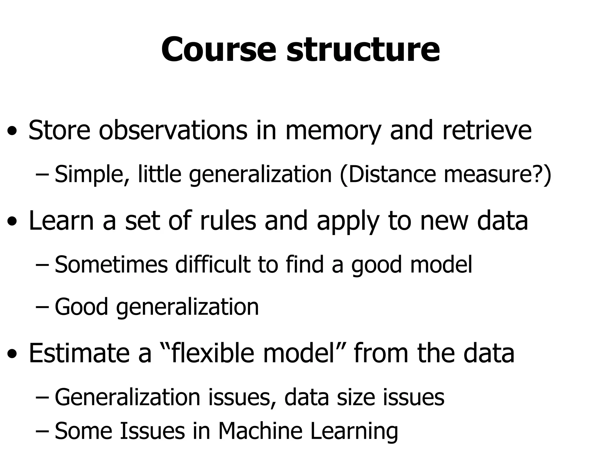
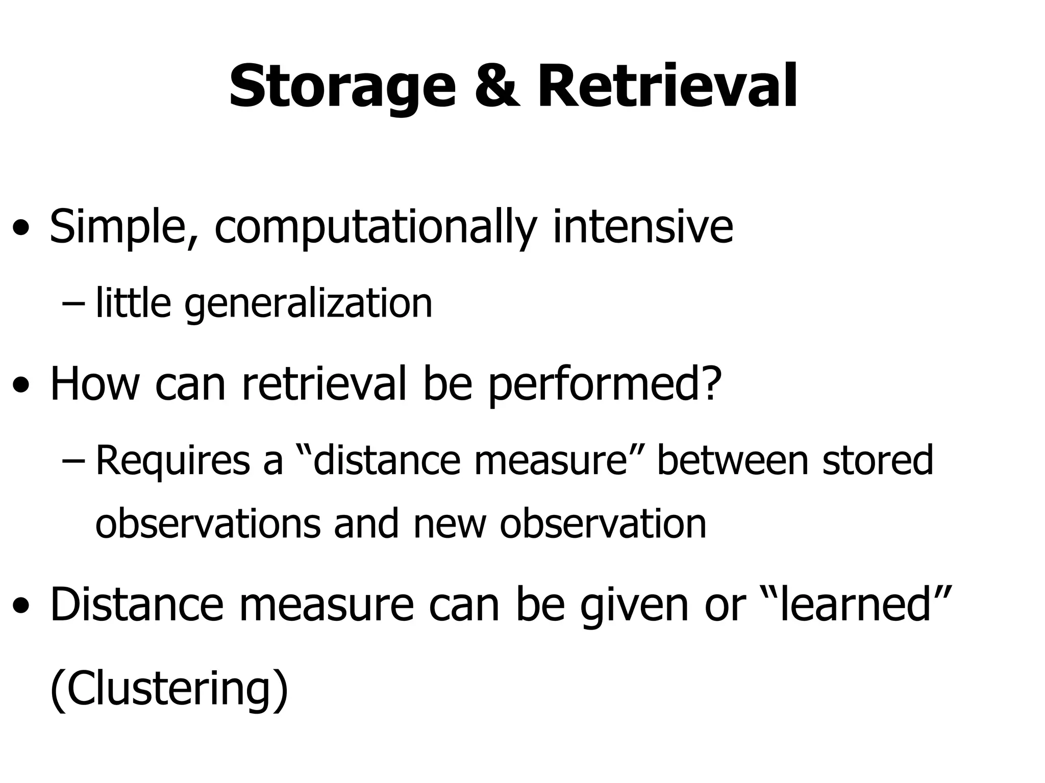
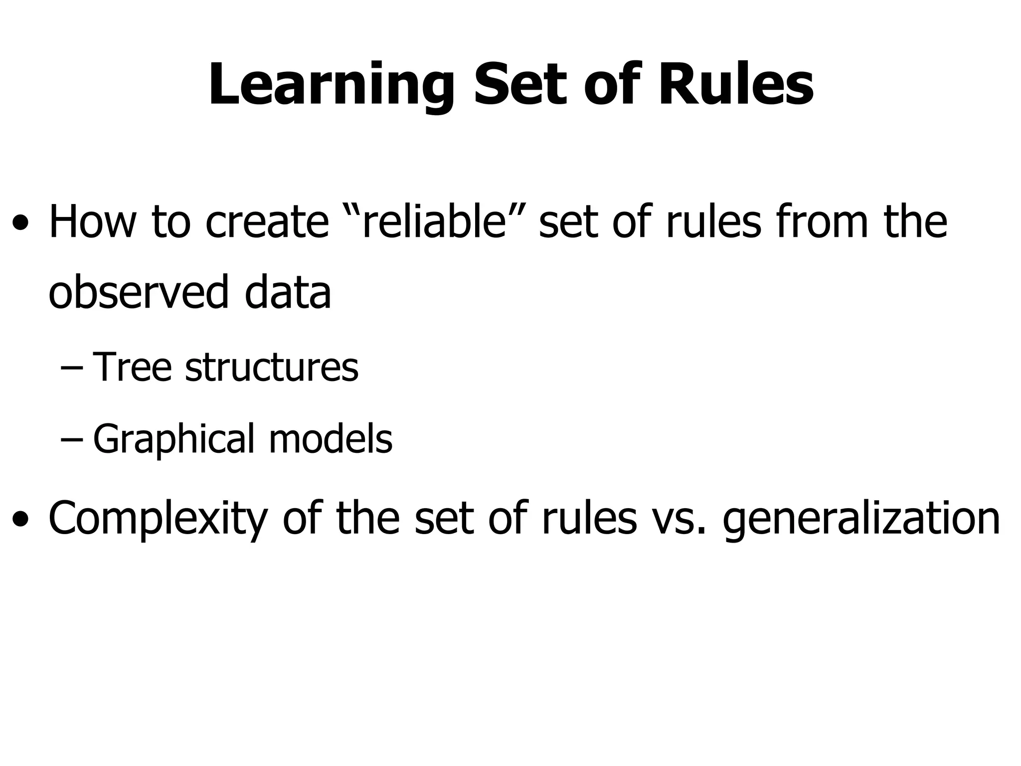
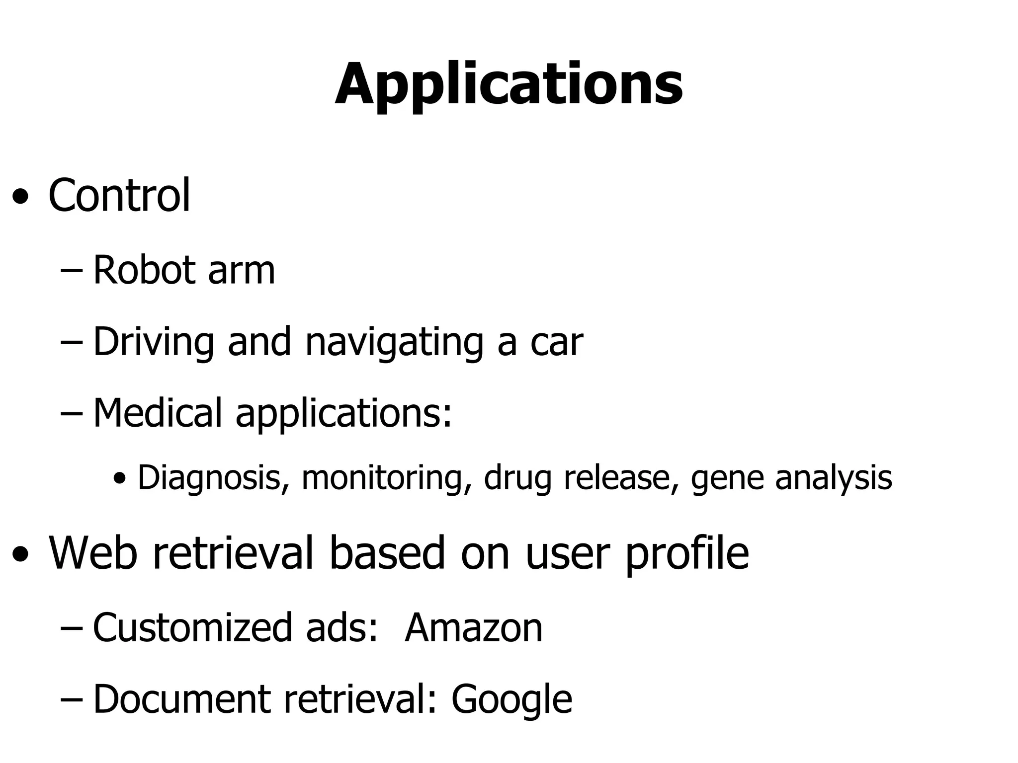
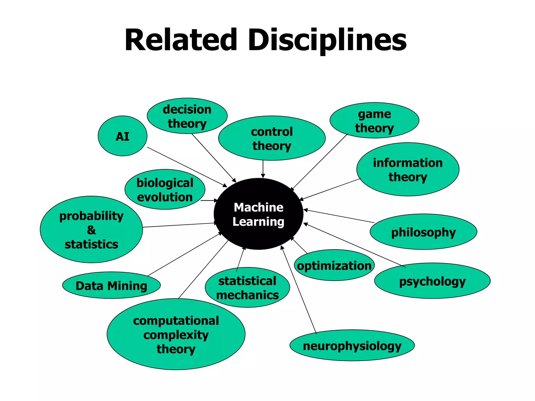
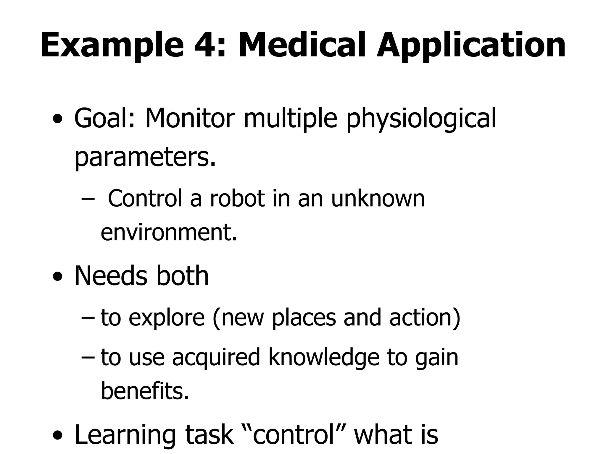
This machine learning course will cover theoretical and practical machine learning concepts. It will include 4 homework assignments and programming in Matlab. Lectures will be supplemented by student-submitted class notes in LaTeX. Topics will include learning approaches like storage and retrieval, rule learning, and flexible model estimation, as well as applications in areas like control, medical diagnosis, and web search. A final exam format has not been determined yet.

1. Machine Learning : Foundations Course Number 0368403401 Prof. Nathan Intrator Teaching Assistants: Daniel Gill, Guy Amit

2. Course structure There will be 4 homework exercises They will be theoretical as well as programming All programming will be done in Matlab Course info accessed from www.cs.tau.ac.il/~nin Final has not been decided yet Office hours Wednesday 4-5 (Contact via email)

3. Class Notes Groups of 2-3 students will be responsible for a scribing class notes Submission of class notes by next Monday (1 week) and then corrections and additions from Thursday to the following Monday 30% contribution to the grade

4. Class Notes (cont’d) Notes will be done in LaTeX to be compiled into PDF via miktex. (Download from School site) Style file to be found on course web site Figures in GIF

5. Basic Machine Learning idea Receive a collection of observations associated with some action label Perform some kind of “Machine Learning” to be able to: Receive a new observation “ Process” it and generate an action label that is based on previous observations Main Requirement: Good generalization

6. Learning Approaches Store observations in memory and retrieve Simple, little generalization (Distance measure?) Learn a set of rules and apply to new data Sometimes difficult to find a good model Good generalization Estimate a “flexible model” from the data Generalization issues, data size issues

7. Storage & Retrieval Simple, computationally intensive little generalization How can retrieval be performed? Requires a “distance measure” between stored observations and new observation Distance measure can be given or “learned” (Clustering)

8. Learning Set of Rules How to create “reliable” set of rules from the observed data Tree structures Graphical models Complexity of the set of rules vs. generalization

9. Estimation of a flexible model What is a “flexible” model Universal approximator Reliability and generalization, Data size issues

10. Applications Control Robot arm Driving and navigating a car Medical applications: Diagnosis, monitoring, drug release, gene analysis Web retrieval based on user profile Customized ads: Amazon Document retrieval: Google

11. Related Disciplines Machine Learning AI probability & statistics computational complexity theory control theory information theory philosophy psychology neurophysiology Data Mining decision theory game theory optimization biological evolution statistical mechanics

12. Example 1: Credit Risk Analysis Typical customer: bank. Database: Current clients data, including: basic profile (income, house ownership, delinquent account, etc.) Basic classification. Goal: predict/decide whether to grant credit.

13. Example 1: Credit Risk Analysis Rules learned from data: IF Other-Delinquent-Accounts > 2 and Number-Delinquent-Billing-Cycles >1 THEN DENY CREDIT IF Other-Delinquent-Accounts = 0 and Income > $30k THEN GRANT CREDIT

14. Example 2: Clustering news Data: Reuters news / Web data Goal: Basic category classification: Business, sports, politics, etc. classify to subcategories (unspecified) Methodology: consider “typical words” for each category. Classify using a “distance “ measure.

15. Example 3: Robot control Goal: Control a robot in an unknown environment. Needs both to explore (new places and action) to use acquired knowledge to gain benefits. Learning task “control” what is observes!

16. Example 4: Medical Application Goal: Monitor multiple physiological parameters. Control a robot in an unknown environment. Needs both to explore (new places and action) to use acquired knowledge to gain benefits. Learning task “control” what is observes!

18. History of Machine Learning 1960’s and 70’s: Models of human learning High-level symbolic descriptions of knowledge, e.g., logical expressions or graphs/networks, e.g., (Karpinski & Michalski, 1966) (Simon & Lea, 1974). Winston’s (1975) structural learning system learned logic-based structural descriptions from examples. Minsky Papert , 1969 1970’s: Genetic algorithms Developed by Holland (1975) 1970’s - present: Knowledge-intensive learning A tabula rasa approach typically fares poorly. “To acquire new knowledge a system must already possess a great deal of initial knowledge.” Lenat’s CYC project is a good example.

19. History of Machine Learning (cont’d) 1970’s - present: Alternative modes of learning (besides examples) Learning from instruction, e.g., (Mostow, 1983) (Gordon & Subramanian, 1993) Learning by analogy, e.g., (Veloso, 1990) Learning from cases, e.g., (Aha, 1991) Discovery (Lenat, 1977) 1991: The first of a series of workshops on Multistrategy Learning (Michalski) 1970’s – present: Meta-learning Heuristics for focusing attention, e.g., (Gordon & Subramanian, 1996) Active selection of examples for learning, e.g., (Angluin, 1987), (Gasarch & Smith, 1988), (Gordon, 1991) Learning how to learn, e.g., (Schmidhuber, 1996)

20. History of Machine Learning (cont’d) 1980 – The First Machine Learning Workshop was held at Carnegie-Mellon University in Pittsburgh. 1980 – Three consecutive issues of the International Journal of Policy Analysis and Information Systems were specially devoted to machine learning. 1981 - Hinton, Jordan, Sejnowski, Rumelhart, McLeland at UCSD Back Propagation alg. PDP Book 1986 – The establishment of the Machine Learning journal. 1987 – The beginning of annual international conferences on machine learning (ICML). Snowbird ML conference 1988 – The beginning of regular workshops on computational learning theory (COLT). 1990’s – Explosive growth in the field of data mining, which involves the application of machine learning techniques.

21. Bottom line from History 1960 – The Perceptron (Minsky Papert) 1960 – “Bellman Curse of Dimensionality” 1980 – Bounds on statistical estimators (C. Stone) 1990 – Beginning of high dimensional data (Hundreds variables) 2000 – High dimensional data (Thousands variables)

22. A Glimpse in to the future Today status: First-generation algorithms: Neural nets, decision trees, etc. Future: Smart remote controls, phones, cars Data and communication networks, software

23. Type of models Supervised learning Given access to classified data Unsupervised learning Given access to data, but no classification Important for data reduction Control learning Selects actions and observes consequences. Maximizes long-term cumulative return.

24. Probability D 1 over and probability D 2 for Equally likely. Computing the probability of “smiley” given a point (x,y). Use Bayes formula. Let p be the probability. Learning: Complete Information (x,y)

25. Task: generate class label to a point at location (x,y) Determine between S or H by comparing the probability of P(S|(x,y)) to P(H|(x,y)). Clearly, one needs to know all these probabilities

26. Predictions and Loss Model How do we determine the optimality of the prediction We define a loss for every prediction Try to minimize the loss Predict a Boolean value. each error we lose 1 (no error no loss.) Compare the probability p to 1/2. Predict deterministically with the higher value. Optimal prediction (for zero-one loss) Can not recover probabilities!

27. Bayes Estimator A Bayes estimator associated with a prior distribution p and a loss function L is an estimator d which minimizes L (p,d). For every x, it is given by d(x), argument of min on estimators d of p (p,d|x). The value r (p) = r (p,dap) is then called the Bayes risk .

28. Other Loss Models Quadratic loss Predict a “real number” q for outcome 1. Loss (q-p) 2 for outcome 1 Loss ([1-q]-[1-p]) 2 for outcome 0 Expected loss: (p-q) 2 Minimized for p=q (Optimal prediction) Recovers the probabilities Needs to know p to compute loss!

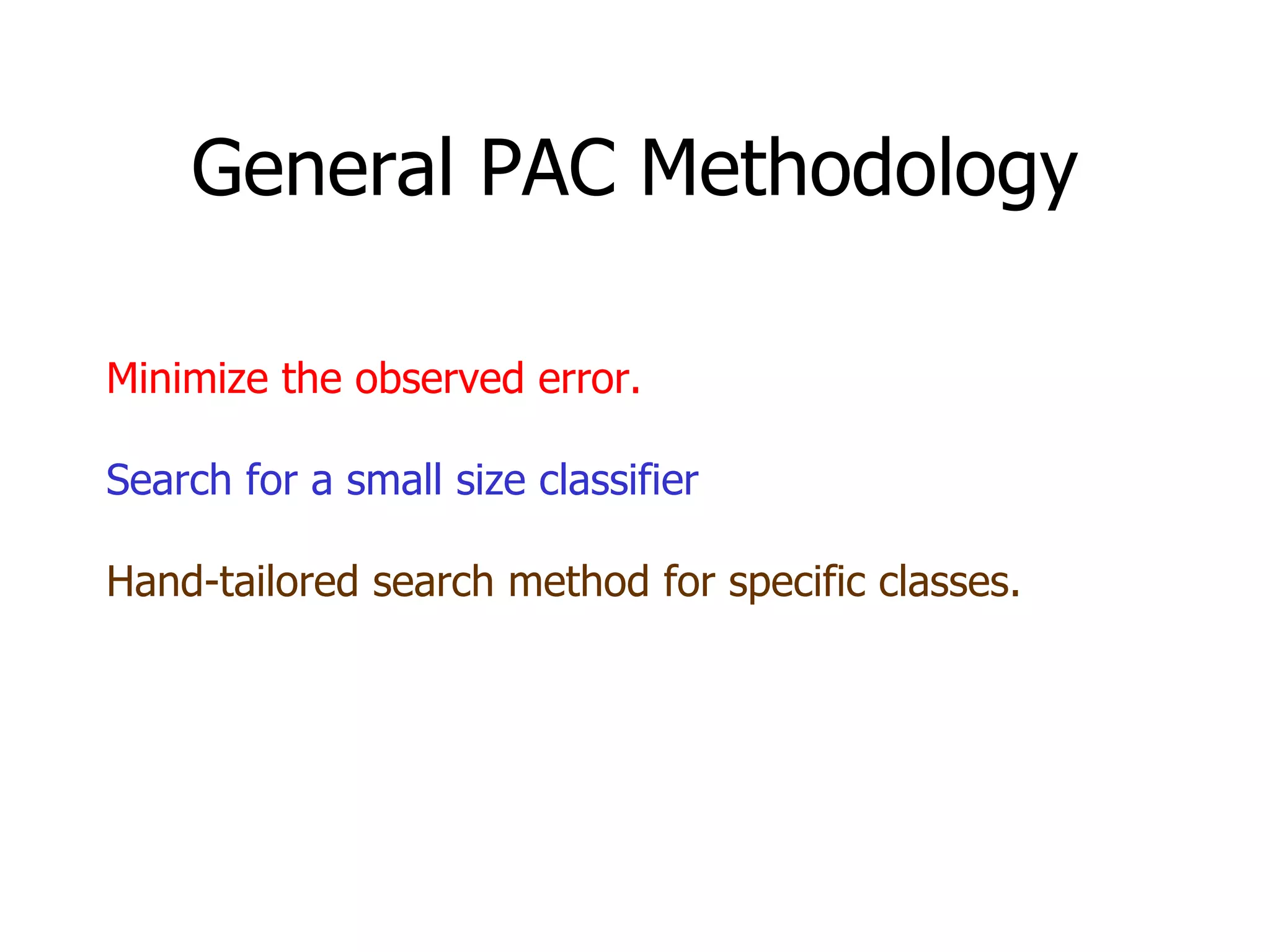
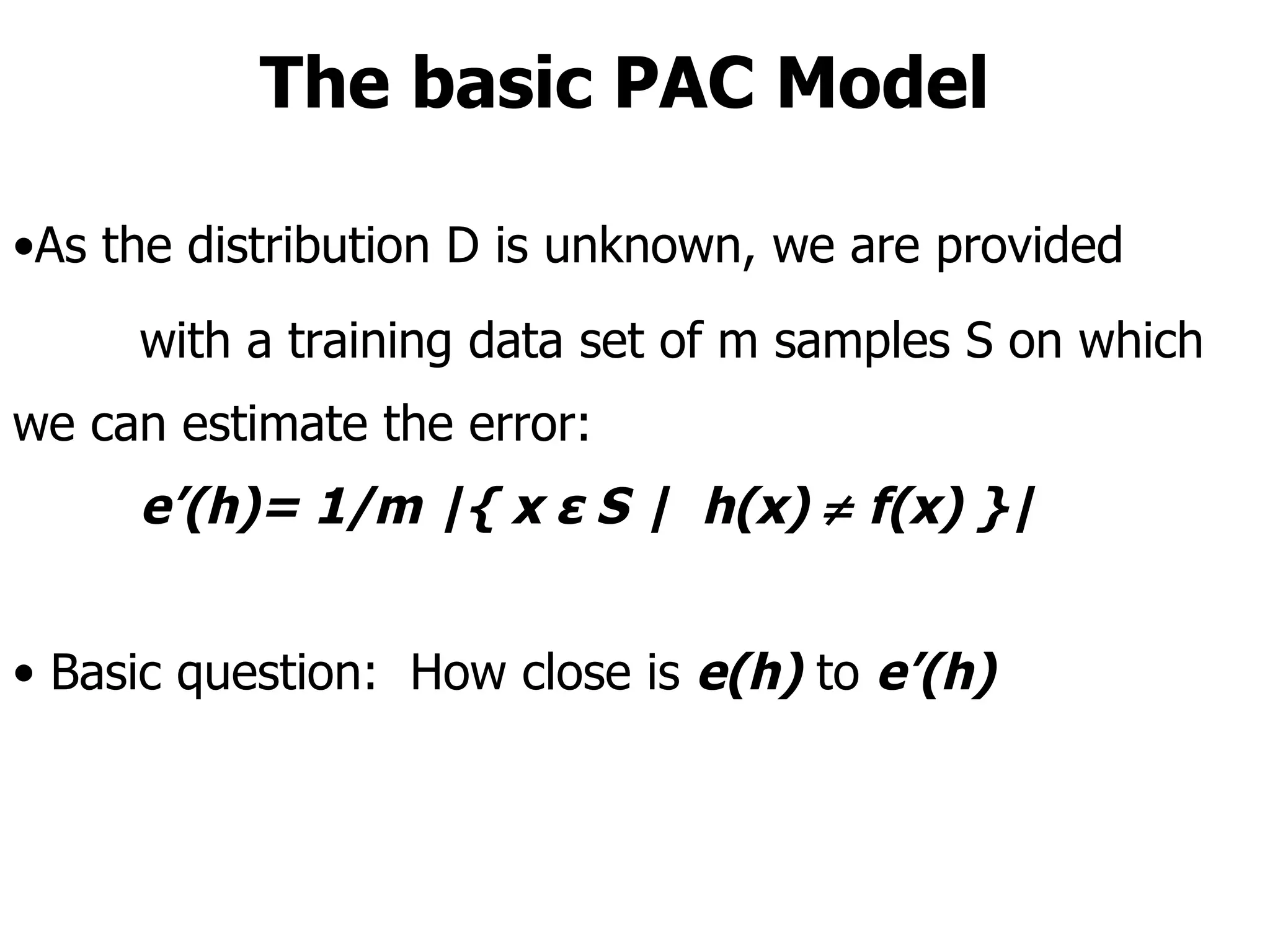
29. The basic PAC Model A batch learning model, i.e., the algorithm is trained over some fixed data set Assumption: Fixed (Unknown distribution D of x in a domain X) The error of a hypothesis h w.r.t. a target concept f is e(h)= Pr D [h(x)≠f(x)] Goal: Given a collection of hypotheses H , find h in H that minimizes e(h).

30. The basic PAC Model As the distribution D is unknown, we are provided with a training data set of m samples S on which we can estimate the error: e’(h)= 1/m |{ x ε S | h(x)  f(x) }| Basic question: How close is e(h) to e’(h)

31. Bayesian Theory Prior distribution over H Given a sample S compute a posterior distribution: Maximum Likelihood (ML) Pr[S|h] Maximum A Posteriori (MAP) Pr[h|S] Bayesian Predictor  h(x) Pr[h|S].

32. Some Issues in Machine Learning What algorithms can approximate functions well, and when? How does number of training examples influence accuracy? How does complexity of hypothesis representation impact it? How does noisy data influence accuracy?

33. More Issues in Machine Learning What are the theoretical limits of learnability? How can prior knowledge of learner help? What clues can we get from biological learning systems? How can systems alter their own representations?

34. Complexity vs. Generalization Hypothesis complexity versus observed error. More complex hypothesis have lower observed error on the training set, Might have higher true error (on test set).

35. Criteria for Model Selection Differ in assumptions about a priori Likelihood of h AIC and BIC are two other theory-based model selection methods Minimum Description Length (MDL)  ’ (h) + |code length of h| Structural Risk Minimization:  ’ (h) + { log |H| / m } ½ m # of training samples

36. Weak Learning Small class of predicates H Weak Learning: Assume that for any distribution D , there is some predicate heH that predicts better than 1/2+e. Multiple Weak Learning Strong Learning

37. Boosting Algorithms Functions: Weighted majority of the predicates. Methodology: Change the distribution to target “hard” examples. Weight of an example is exponential in the number of incorrect classifications. Good experimental results and efficient algorithms.

38. Computational Methods How to find a hypothesis h from a collection H with low observed error. Most cases computational tasks are provably hard. Some methods are only for a binary h and others for both.

40. Nearest Neighbor Methods Classify using near examples. Assume a “structured space” and a “metric” + + + + - - - - ?

41. Separating Hyperplane Perceptron: sign(  x i w i ) Find w 1 .... w n Limited representation x 1 x n w 1 w n  sign

42. Neural Networks Sigmoidal gates : a=  x i w i and output = 1/(1+ e -a ) Learning by “Back Propagation” of errors x 1 x n

43. Decision Trees x 1 > 5 x 6 > 2 +1 +1 -1

44. Decision Trees Top Down construction: Construct the tree greedy, using a local index function. Ginni Index : G(x) = x(1-x), Entropy H(x) ... Bottom up model selection: Prune the decision Tree while maintaining low observed error.

45. Decision Trees Limited Representation Highly interpretable Efficient training and retrieval algorithm Smart cost/complexity pruning Aim: Find a small decision tree with a low observed error.

46. Support Vector Machine n dimensions m dimensions

47. Support Vector Machine Use a hyperplane in the LARGE space. Choose a hyperplane with a large MARGIN. + + + + - - - Project data to a high dimensional space.

48. Reinforcement Learning Main idea: Learning with a Delayed Reward Uses dynamic programming and supervised learning Addresses problems that can not be addressed by regular supervised methods E.g., Useful for Control Problems. Dynamic programming searches for optimal policies.

49. Genetic Programming A search Method. Local mutation operations Cross-over operations Keeps the “best” candidates Change a node in a tree Replace a subtree by another tree Keep trees with low observed error Example: decision trees

50. Unsupervised learning: Clustering

51. Unsupervised learning: Clustering

52. Basic Concepts in Probability For a single hypothesis h: Given an observed error Bound the true error Markov Inequality

53. Basic Concepts in Probability Chebyshev Inequality

54. Basic Concepts in Probability Chernoff Inequality i.i.d, Convergence rate of empirical mean to the true mean

56. Basic Concepts in Probability Switching from h 1 to h 2 : Given the observed errors Predict if h 2 is better. Total error rate Cases where h 1 (x)  h 2 (x) More refine

57. Course structure Store observations in memory and retrieve Simple, little generalization (Distance measure?) Learn a set of rules and apply to new data Sometimes difficult to find a good model Good generalization Estimate a “flexible model” from the data Generalization issues, data size issues Some Issues in Machine Learning ffl What algorithms can approximate functions well (and when)? ffl How does number of training examples influence accuracy? ffl How does complexity of hypothesis representation impact it? ffl How does noisy data influence accuracy? ffl What are the theoretical limits of learnability? ffl How can prior knowledge of learner help? ffl What clues can we get from biological learning systems? ffl How can systems alter their own representations? 21 lecture slides for textbook Machine Learning, T. Mitchell, McGraw Hill, 1997

58. Fourier Transform f(x) =  z  z (x)  z (x) = (-1) <x,z> Many Simple classes are well approximated using large coefficients. Efficient algorithms for finding large coefficients.

59. General PAC Methodology Minimize the observed error. Search for a small size classifier Hand-tailored search method for specific classes.

60. Other Models Membership Queries x f(x)