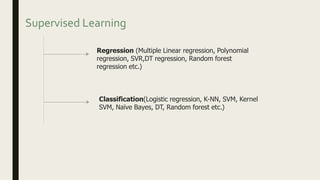
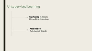
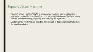
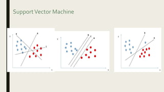
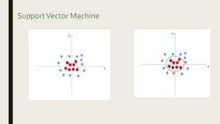
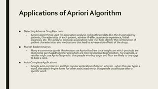
SlideShare a Scribd company logo
PRIMER ON MAJOR
DATA MINING
ALGORITHMS
Vikram Singh Sankhala
What is Data Mining
■ Data mining is the process of discovering or extracting new patterns from large data
sets involving methods from
– Statistics
– Artificial intelligence.
MajorTechniques Used
■ Classification
■ Regression
■ Clustering
■ Association Rules
■ PrincipalComponentsAnalysis
Supervised Learning
Regression (Multiple Linear regression, Polynomial
regression, SVR,DT regression, Random forest
regression etc.)
Classification(Logistic regression, K-NN, SVM, Kernel
SVM, Naïve Bayes, DT, Random forest etc.)
Unsupervised Learning
Clustering (K-means,
Hierarchical clustering)
Association
Rule(Apriori, Eclast)
SupportVector Machine
• “Support Vector Machine” (SVM) is a supervised machine learning algorithm
which can be used for both classification or regression challengesThe Data Mining
Process include collecting, exploring and selecting the right data.
• Support Vector Machines are based on the concept of decision planes that define
decision boundaries.
SupportVector Machine
Advantage of SVM
• Performance is good when linear problems
• It doesn't work on nonlinear problems (you need Kernel SVM) and
you cannot get the probabilities of the classes.
Disadvantage of SVM
SupportVector Machine Application
• SVM has been used successfully in many real-world problems
- text (and hypertext) categorization
- image classification
- bioinformatics (Protein classification,
Cancer classification)
- hand-written character recognition
Naïve Bayes Algorithm
• It is a classification technique based on Bayes’ Theorem with an
assumption of independence among predictors.
• Naive Bayes model is easy to build and particularly useful for very
large data sets (not feature wise).
Advantage of Naïve Bayes
• You can get the probabilities of the classes and that it works on non
linear problems
• It doesn't work properly on datasets with many features
Disadvantage of Naïve Bayes
Naïve Bayes Application
• Spam Classification
• Given an email, predict whether it is spam or not
• Medical Diagnosis
• Given a list of symptoms, predict whether a patient has disease X
or not
• Weather
• Based on temperature, humidity, etc… predict if it will rain
tomorrow
• Text classification/ Spam Filtering/ Sentiment Analysis
DecisionTree and Random Forest
• Decision Tree - Decision tree is a type of supervised learning
algorithm (having a pre-defined target variable) that is mostly used
in classification problems.
• It works for both categorical and continuous input and output
variables.
Random Forest
• Random forest is an ensemble classifier made using many decision
tree
• Ensemble Model – Combines the results from different models &
produce better results.
Advantage and Disadvantage of DT and Random Forest
• Advantage –
• Easy to Understand
• Useful in Data exploration
• Less data cleaning required
• Handle both numerical and categorical variables
• Disadvantage –
• Over fitting
• Not fit for continuous variables
Application of DT and Random Forest
• Astronomy:
• star-galaxy classification, determining galaxy counts.
• Biomedical Engineering:
• Use of decision trees for identifying features to be used in
implantable devices can be found
• Pharmacology:
• Use of tree based classification for drug analysis
• Manufacturing:
• Chemical material evaluation for manufacturing and production
• Medicine:
• Analysis of the Sudden Infant Death Syndrome
Which Model….?
• DT - when you want to have clear interpretation of your model results
• Random Forest - when you are just looking for high performance
with less need for interpretation
• SVM - when your business problem is a linear problem (with a linearly
separable dataset)
• Naive Bayes - when you want your business problem to be based on
a probabilistic approach. For example if you want to rank your
customers from the highest probability to buy a certain product, to
the lowest.
Cluster Analysis (Unsupervised Learning)
• Clustering analysis is the task of grouping a set of objects in such a
way that objects in the same group (called a cluster) are more similar
(in some sense or another) to each other than to those in other
groups (clusters).
Advantage of Clustering (K-means)
• If variables are huge, then K-Means most of the times
computationally faster than hierarchical clustering
• K-Means produce tighter clusters than hierarchical clustering
• Difficult to predict K-Value
Disadvantage of Clustering (K-means)
Clustering Application
• Marketing:
• Discovering distinct groups in customer databases.
• Insurance:
• Identifying groups of crop insurance policy holders with a high
average claim rate. Farmers crash crops, when it is “profitable”.
• Land use:
• Identification of areas of similar land use in a GIS database.
• Seismic studies:
• Identifying probable areas for oil/gas exploration based on
seismic data.
Classification
1. Decision trees
2. CART: Classification and Regression Trees
3. Ruleset classifiers
4. Ensemble Classifiers
5. Support vector machines
6. Naive Bayes
Decision trees
■ Decision tree builds classification or regression models in the form of a tree structure.
■ Decision nodes and leaf nodes
■ Decision node has two or more branches
■ Leaf node represents a classification or decision
TheAlgorithms used in the decision trees are ID3 , C4.5,
CART, C5.0, CHAID, QUEST, CRUISE, etc.
■ The splitting of nodes is decided by algorithms like information gain, chi square, Gini
index.
■ ID3, or Iterative Dichotomizer, was the first of three DecisionTree implementations
developed by Ross Quinlan
■ The ID3 algorithm uses a greedy search. It selects a test using the information gain
criterion (Minimizing Shannon Entropy), and then never explores the possibility of
alternate choices.
'Greedy Algorithm'?
■ Makes a locally-optimal choice in the hope that this choice will lead to a globally-
optimal solution.
■ A code is a mapping from a “string” (a finite sequence of letters) to a finite sequence of
binary numbers.
■ The goal of compression algorithms is to encode strings with the smallest sequence of
binary numbers.
■ Shannon entropy gives the optimal compression rate, that can be approached but not
improved.
■ Information Gain is inversely Proportion to entropy.
■ The Greedy Algorithm is used at each node to arrive at the next node.
Information Gain and Shannon Entropy
■ Suppose you need to uncover a certain English word of five letters.
■ You manage to obtain one letter, namely an e.This is useful information, but the letter
e is common in English, so this provides little information.
■ If, on the other hand, the letter that you discover is j (the least common in English), the
search has been more narrowed and you have obtained more information.
■ The unit for the information gain is the bit.
CART
■ ClassificationTrees
■ RegressionTrees
ClassificationTrees
■ These are considered as the default kind of decision trees used to separate a dataset
into different classes, based on the response variable.These are generally used when
the response variable is categorical in nature.
RegressionTrees
■ When the response or target variable is continuous or numerical, regression trees are
used.These are generally used in predictive type of problems when compared to
classification
C5.0 model
■ A C5.0 algorithm is used to build either a decision tree or a rule set
■ A C5.0 model works by splitting the sample based on the field that provides the
maximum information gain.
Applications of DecisionTree Machine
LearningAlgorithm
■ Decision trees are among the popular machine learning algorithms that find great use
in finance for option pricing.
■ Remote sensing is an application area for pattern recognition based on decision trees.
■ Decision tree algorithms are used by banks to classify loan applicants by their
probability of defaulting payments.
Libraries
■ The Data Science libraries in Python language to implement DecisionTree Machine
LearningAlgorithm are – SciPy and Sci-Kit Learn.
■ The Data Science libraries in R language to implement DecisionTree Machine Learning
Algorithm is caret.
Random Forest
■ It is a type of ensemble machine learning algorithm called Bootstrap Aggregation or
bagging.
Bootstrap Method
■ Let’s assume we have a sample of 100 values (x) and we’d like to get an estimate of the
mean of the sample
■ Create many (e.g. 1000) random sub-samples of our dataset with replacement
(meaning we can select the same value multiple times).
■ Calculate the mean of each sub-sample.
■ Calculate the average of all of our collected means and use that as our estimated
mean for the data.
Bootstrap Aggregation (Bagging)
■ Bagging of the CART algorithm would work as follows.
– Create many (e.g. 100) random sub-samples of our dataset with replacement.
– Train a CART model on each sample.
– Given a new dataset, calculate the average prediction from each model.
Applications of Random Forest
Algorithms
■ Random Forest algorithms are used by banks to predict if a loan applicant is a likely
high risk.
■ They are used in the automobile industry to predict the failure or breakdown of a
mechanical part.
■ These algorithms are used in the healthcare industry to predict if a patient is likely to
develop a chronic disease or not.
■ They can also be used for regression tasks like predicting the average number of social
media shares and performance scores.
■ Recently, the algorithm has also made way into predicting patterns in speech
recognition software and classifying images and texts.
Random Forest and CART
■ Even with Bagging, the decision trees (CART) can have a lot of structural similarities
and in turn have high correlation in their predictions.
■ To reduce Correlation between features, the random forest algorithm changes the
procedure so that the learning algorithm is limited to a random sample of features of
which to search.
■ The number of features that can be searched at each split point (m) must be specified
as a parameter to the algorithm.
Libraries
■ Data Science libraries in Python language to implement Random Forest Machine
LearningAlgorithm is Sci-Kit Learn.
■ Data Science libraries in R language to implement Random Forest Machine Learning
Algorithm is randomForest.
Naïve Bayes
■ A Naive Bayes classifier assumes that the presence of a particular feature in a class is
unrelated to the presence of any other feature.
■ For example, a fruit may be considered to be an apple if it is red, round, and about 3
inches in diameter.
■ Even if these features depend on each other or upon the existence of the other
features, all of these properties independently contribute to the probability that this
fruit is an apple
■ That is why it is known as ‘Naive’.
■ This algorithm is mostly used in text classification and with problems having multiple
classes.
How Naive Bayes algorithm works
■ Step 1: Convert the data set into a frequency table
■ Step 2: Create Likelihood table by finding the probabilities
■ Step 3: Now, use Naive Bayesian equation to calculate the posterior probability for
each class.
■ Step 4:The class with the highest posterior probability is the outcome of prediction.
Applications of Naive Bayes Algorithms
■ Real time Prediction
■ Multi class Prediction
■ Text classification/ Spam Filtering/ Sentiment Analysis Recommendation
System: Naive Bayes Classifier and Collaborative Filtering together builds a
Recommendation System that uses machine learning and data mining techniques to
filter unseen information and predict whether a user would like a given resource or not
■ Disease prediction
■ Document classification
SupportVector Machines
■ In a two-class learning task, the aim of SVM is to find the best classification function to
distinguish between members of the two classes in the training data.
■ For a linearly separable dataset, a linear classification function corresponds to a
separating hyperplane f (x ) that passes through the middle of the two classes,
separating the two.
Margin Maximization
■ In case of multiple classes, SVM works by classifying the data into different classes by
finding a line (hyperplane) which separates the training data set into classes.
■ As there are many such linear hyperplanes, SVM algorithm tries to maximize the
distance between the various classes that are involved and this is referred as margin
maximization.
■ If the line that maximizes the distance between the classes is identified, the
probability to generalize well to unseen data is increased.
SVM can also be used for
■ Regression – By minimizing the error between actual and Predicted value to be within
a margin Epsilon
■ Ranking
SVM’s are classified into two categories:
■ Linear SVM’s – In linear SVM’s the training data i.e. classifiers are separated by a
hyperplane.
■ Non-Linear SVM’s- In non-linear SVM’s it is not possible to separate the training data
using a hyperplane.
Applications
■ Risk assessment
■ Stock Market forecasting
■ Most commonly, SVM is used to compare the performance of a stock with other
stocks in the same sector.This helps companies make decisions about where they
want to invest.
Association Analysis
■ Association rule implies that if an item A occurs, then item B also occurs with a certain
probability.
The Apriori algorithm
■ The approach is to find frequent item sets from a transaction dataset and derive
association rules
■ A ratio is derived like out of the 100 people who purchased an apple, 85 people also
purchased an orange.
Libraries -The Apriori algorithm
■ Data Science Libraries in Python to implement Apriori Machine LearningAlgorithm –
There is a python implementation for Apriori in PyPi
■ Data Science Libraries in R to implement Apriori Machine LearningAlgorithm – arules
Applications of Apriori Algorithm
■ Detecting Adverse Drug Reactions
– Apriori algorithm is used for association analysis on healthcare data like-the drugs taken by
patients, characteristics of each patient, adverse ill-effects patients experience, initial
diagnosis, etc.This analysis produces association rules that help identify the combination of
patient characteristics and medications that lead to adverse side effects of the drugs.
■ Market Basket Analysis
– Many e-commerce giants like Amazon useApriori to draw data insights on which products are
likely to be purchased together and which are most responsive to promotion. For example, a
retailer might useApriori to predict that people who buy sugar and flour are likely to buy eggs
to bake a cake.
■ Auto-CompleteApplications
– Google auto-complete is another popular application of Apriori wherein - when the user types a
word, the search engine looks for other associated words that people usually type after a
specific word.
clustering
1. The EM algorithm
2. The k-means algorithm
3. k-nearest neighbor classification
The Expectation–Maximization algorithm
■ The EM algorithm attempts to approximate the observed distributions of values based
on mixtures of different distributions in different clusters.
■ The EM clustering algorithm then computes probabilities of cluster memberships
based on one or more of the mixture of probability distributions.
The k-means algorithm
1. Randomly select ‘c’ cluster centers.
2. Calculate the distance between each data point and cluster centers.
3. Assign the data point to the cluster center whose distance from the cluster center is
minimum of all the cluster centers.
4. Recalculate the new cluster center using the algorithm (aims at minimizing an objective
function know as squared error function).
5. Recalculate the distance between each data point and new obtained cluster centers.
6. If no data point was reassigned then stop, otherwise repeat from step (3).
7. This learning algorithm requires prior specification of the number of cluster centers.
Applications
■ Search engines likeYahoo and Bing (to identify relevant results)
■ Data libraries
■ Google image search
k-nearest neighbor classification
■ Used for classification and regression
■ The number k will have to be specified
■ The kNN algorithm will search through the training dataset for the k-most similar
instances.
■ This is a process of calculating the distance for all instances and selecting a subset with
the smallest distance values..
Applications
■ Pattern recognition (like to predict how cancer may spread)
■ Statistical estimation (like to predict if someone may default on a loan)
Linear Regression
■ “Ordinary least squares” strategy
■ Draw a line, and then for each of the data points, measure the vertical distance
between the point and the line, and add these up;
■ The fitted line would be the one where this sum of distances is as small as possible
Logistic Regression
■ Binary Logistic Regression –The most commonly used logistic regression when the
categorical response has 2 possible outcomes i.e. either yes or not. Example –
Predicting whether a student will pass or fail an exam, predicting whether a student
will have low or high blood pressure, predicting whether a tumor is cancerous or not.
■ Multi-nominal Logistic Regression - Categorical response has 3 or more possible
outcomes with no ordering. Example- Predicting what kind of search engine (Yahoo,
Bing,Google, and MSN) is used by majority of US citizens.
■ Ordinal Logistic Regression - Categorical response has 3 or more possible outcomes
with natural ordering. Example- How a customer rates the service and quality of food
at a restaurant based on a scale of 1 to 10.
Logistic Regression
■ It measures the relationship between the categorical dependent variable and one or
more independent variables by estimating probabilities using a logistic function, which
is the cumulative logistic distribution.
■ regressions can be used in real-world applications such as:
– Credit Scoring
– Measuring the success rates of marketing campaigns
– Predicting the revenues of a certain product
Boosting
■ In 1988, Kearns andValiant posed an interesting question, i.e., whether a weak
learning algorithm that performs just slightly better than random guess could be
“boosted” into an arbitrarily accurate strong learning algorithm.
■ AdaBoost was born with in response to this question.AdaBoost has given rise to
abundant research on theoretical aspects of ensemble methods, which can be easily
found in machine learning and statistics literature.
■ It is worth mentioning that for their AdaBoost paper, Schapire and Freund won the
Godel Prize, which is one of the most prestigious awards in theoretical computer
science, in the year of 2003.
How Adaboost works
■ First, it assigns equal weights to all the training examples (xi , yi )(i ∈ {1,..., m}). Denote the
distribution of the weights at the t -th learning round as Dt
■ From the training set and Dt the algorithm generates a weak or base learner ht : X →Y by
calling the base learning algorithm.
■ Then, it uses the training examples to test ht , and the weights of the incorrectly classified
examples will be increased.Thus, an updated weight distribution Dt +1 is obtained.
■ From the training set and Dt +1 AdaBoost generates another weak learner by calling the
base learning algorithm again.
■ Such a process is repeated forT rounds, and the final model is derived by weighted
majority voting of theT weak learners, where the weights of the learners are determined
during the training process.
Artificial Neural Networks
■ Artificial Neural Networks are named so because they’re based on the structure and
functions of real biological neural networks.
■ Information flows through the network and in response, the neural network changes
based on the input and output.
■ Applications
– Character recognition (understanding human handwriting and converting it to
text)
– Image compression
– Stock market prediction
– Loan applications
Linear Discriminant Analysis
■ Linear discriminant analysis (LDA) and the related Fisher’s linear discriminant are
methods used in statistics, pattern recognition and machine learning to find a linear
combination of features which characterizes or separates two or more classes of
objects or events.
■ The resulting combination may be used as a linear classifier, or, more commonly, for
dimensionality reduction before later classification.
■ QDA is a general discriminant function with a quadratic decision boundaries which can
be used to classify datasets with two or more classes.
Method
■ LDA is based upon the concept of searching for a linear combination of variables
(predictors) that best separates two classes (targets)
■ To capture the notion of separability, Fisher defined the following score function.
■ Given the score function, the problem is to estimate the linear coefficients that
maximize the score function.
■ One way of assessing the effectiveness of the discrimination is to calculate
the Mahalanobis distance between two groups. A distance greater than 3 means that
in two averages differ by more than 3 standard deviations. It means that the overlap
(probability of misclassification) is quite small.
Predictors Contribution
■ A simple linear correlation between the model scores and predictors can be used to
test which predictors contribute significantly to the discriminant function. Correlation
varies from -1 to 1, with -1 and 1 meaning the highest contribution but in different
directions and 0 means no contribution at all.
Applications of LDA
■ Bankruptcy prediction: In bankruptcy prediction based on accounting ratios and other
financial variables, linear discriminant analysis was the first statistical method applied
to systematically explain which firms entered bankruptcy vs. survived.
■ Marketing: In marketing, discriminant analysis was once often used to determine the
factors which distinguish different types of customers and/or products on the basis of
surveys or other forms of collected data.
■ Biomedical studies:The main application of discriminant analysis in medicine is the
assessment of severity state of a patient and prognosis of disease outcome.
The Gradient Descent algorithm
■ Gradient descent is an optimization algorithm used to find the values of parameters
(coefficients) of a function (f) that minimizes a cost function (cost).
■ The goal is to continue to try different values for the coefficients, evaluate their cost
and select new coefficients that have a slightly better (lower) cost.
How itWorks
■ The procedure starts off with initial values for the coefficient or coefficients for the
function.These could be 0.0 or a small random value.
■ The cost of the coefficients is evaluated by plugging them into the function and
calculating the cost
■ The derivative of the cost is calculated.The derivative is a concept from calculus and
refers to the slope of the function at a given point.We need to know the slope so that
we know the direction (sign) to move the coefficient values in order to get a lower cost
on the next iteration
■ Now that we know from the derivative which direction is downhill, we can now update
the coefficient values.
Cont.
■ A learning rate parameter (alpha) must be specified that controls how much the
coefficients can change on each update.
■ delta = derivative(cost)
■ coefficient = coefficient – (alpha * delta)
■ This process is repeated until the cost of the coefficients (cost) is 0.0 or close enough
to zero to be good enough.
Applications
■ Common examples of algorithms with coefficients that can be optimized using
gradient descent are
– Linear Regression and
– Logistic Regression.
State of the Art Algorithms
■ XGBoost for Classification and Regression.
■ Convolutional Neural Networks for Image Classification.
■ DBSCAN for Clustering
■ Collaborative Filtering for Recommender Systems
■ SVD++ for Recommender Systems
■ NMF for Dimensionality Reduction
■ Deep Autoencoders for deep learning systems and to find the best set of features to represent a dataset
■ Sparse Filtering for Representation
■ Hash Kernels for Representation
■ T-SNE to visualize multidimensional datasets
■ LSTMs forTime Series and Sequences. Applications in Sentiment Analysis.
■ MCMC and Metropolis Hastings Algorithm.
XGBoost for Classification and
Regression
■ The XGBoost library implements the gradient boosting decision tree algorithm.
■ Boosting is an ensemble technique where new models are added to correct the errors
made by existing models. Models are added sequentially until no further
improvements can be made.
■ It gives more weight to the misclassified points sequentially for every model.
■ The Final Model is a weighted combination of the weak classifiers
■ You are updating your model using gradient descent and hence the name, gradient
boosting.
Convolutional Neural Networks for
Image Classification
■ CNNs have wide applications in image and video recognition, recommender systems
and natural language processing.
■ CNNs, like neural networks, are made up of neurons with learnable weights and
biases. Each neuron receives several inputs, takes a weighted sum over them, pass it
through an activation function and responds with an output.
■ Convolutional networks perform optical character recognition (OCR) to digitize text
and make natural-language processing possible on analog and hand-written
documents.
■ Convolutional neural networks ingest and process images as tensors.
Contd.
■ A tensor encompasses the dimensions beyond that 2-D plane e.g. a 2 x 3 x 2 tensor.
■ Tensors are formed by arrays nested within arrays, and that nesting can go on
infinitely, accounting for an arbitrary number of dimensions far greater than what we
can visualize spatially.
■ Convolutional networks pass many filters over a single image, each one picking up a
different signal.Therefore convolutional nets learn images in pieces that we call
feature maps.
DBSCAN for Clustering
■ It stands for Density Based SpatialClustering of applications with Noise
■ it groups together points that are closely packed together (points with many nearby
neighbors), marking as outliers points that lie alone in low-density regions (whose
nearest neighbors are too far away)
■ The two parameters we need to specify are:
■ What is the minimum number of data points needed to determine a single cluster
■ How far away can one point be from the next point within the same cluster - Epsilon
Collaborative Filtering for Recommender
Systems
■ Collaborative filtering, also referred to as social filtering, filters information by using
the recommendations of other people.
■ Most collaborative filtering systems apply the so called neighborhood-based
technique.
■ In the neighbourhood-based approach a number of users is selected based on their
similarity to the active user.
■ A prediction for the active user is made by calculating a weighted average of the
ratings of the selected users.
SVD++ for Recommender Systems
■ Matrix factorization algorithms work by decomposing the user-item interaction matrix
into the product of two lower dimensionality rectangular matrices.
■ SVD consists of factorization two lower dimensional matrices, the first one has a row
for each user, while the second has a column for each item.
■ The row or column associated to a specific user or item is referred to as latent factors.
■ Increasing the number of latent factor will improve personalization, therefore
recommendation quality, until the number of factors becomes too high, at which point
the model starts to overfit and the recommendation quality will decrease
■ SVD++ is a matrix factorization method with implicit feedback.
■ It exploit all available interactions both explicit (e.g. numerical ratings) and implicit
(e.g. likes, purchases, skipped, bookmarked).
NMF for Dimensionality Reduction
■ Non-negative matrix factorization is an important method in the analysis of high
dimensional datasets.
■ Principal component analysis (PCA) and singular value decomposition (SVD) are
popular techniques for dimensionality reduction based on matrix decomposition,
■ However they contain both positive and negative values in the decomposed matrices.
■ Since matrices decomposed by NMF only contain non-negative values, the original
data are represented by only additive, not subtractive, combinations of the basis
vectors.
Deep Auto Encoders
■ An Autoencoder is a feedforward neural network having an input layer, one hidden
layer and an output layer.
■ The transition from the input to the hidden layer is called the encoding step and the
transition from the hidden to the output layer is called the decoding step.
■ A DeepAutoencoder has multiple hidden layers.
■ The additional hidden layers enable the Autoencoder to learn mathematically more
complex underlying patterns in the data.
Sparse Filtering
■ Traditionally, feature learning methods have largely sought to learn models that
provide good approximations of the true data distribution
■ Sparse Filtering is a form of unsupervised feature learning that learns a sparse
representation of the input data without directly modelling it.
■ It has only has only one hyperparameter, the number of features to learn.
■ Sparse filtering scales gracefully to handle high-dimensional inputs,
t-SNE to visualize multidimensional datasets
■ t-SNE stands for t-Distributed Stochastic Neighbour Embedding and its main aim is
that of dimensionality reduction.
■ The dimensionality of a set of images is the number of pixels in any image, which
ranges from thousands to millions.We need to reduce the dimensionality of a dataset
from an arbitrary number to two or three.
■ Stochastic neighbour embedding techniques compute an N ×N similarity matrix in
both the original data space and in the low-dimensional embedding space called
Similarity Matrices.
Contd.
■ The distribution over pairs of objects is defined such that pairs of similar objects have a
high probability under the distribution, whilst pairs of dissimilar points have a low
probability.
■ The probabilities are generally given by a normalizedGaussian or Student-t kernel
computed from the data space or from the embedding space.
■ The low-dimensional embedding is learned by minimizing the Kullback-Leibler
divergence between the two probability distributions (computed in the original data
space and the embedding space) with respect to the locations of the points in the
embedding space.
■ This is the topic of manifold learning, also called nonlinear dimensionality reduction, a
branch of machine learning (more specifically, unsupervised learning).
■ It is still an active area of research today and tries to develop algorithms that can
automatically recover a hidden structure in a high-dimensional dataset.
LSTMs forTime Series and Sequences
■ A usual RNN (Recurrent Neural Network) has a short-term memory. In combination
with a LSTM they also have a long-term memory
■ An LSTM unit is composed of a cell, an input gate, an output gate and a forget gate.
■ The cell remembers values over arbitrary time intervals and the three gates regulate
the flow of information into and out of the cell.
■ LSTM’s enable Recurrent Neural Networks to remember their inputs over a long
period of time.
MCMC and Metropolis Algorithm
■ The Metropolis–Hastings algorithm is a Markov chain Monte Carlo (MCMC) method
for obtaining a sequence of random samples from multi-dimensional distributions,
especially when the number of dimensions is high.
■ The algorithm proceeds by generating random numbers over a unform distribution
and uses an accept or reject criteria.
■ If the criteria is accepted, the a transition is made over a StochasticTransition Matrix.
■ It uses the property of an Ergodicity of a Markov Process to ensure that the probability
of reaching any point in the space is greater than Zero.
■ A stochastic process is said to be ergodic if its statistical properties can be deduced
from a single, sufficiently long, random sample of the process.
■ The reasoning is that any collection of random samples from a process must represent
the average statistical properties of the entire process.
■ The End

More Related Content

What's hot

Classification
ClassificationClassification
Classification
DataminingTools Inc
 
Decision tree
Decision treeDecision tree
Decision tree
ShraddhaPandey45
 
Machine Learning Real Life Applications By Examples
Machine Learning Real Life Applications By ExamplesMachine Learning Real Life Applications By Examples
Machine Learning Real Life Applications By Examples
Mario Cartia
 
6 module 4
6 module 46 module 4
6 module 4
tafosepsdfasg
 
Data Mining: Mining stream time series and sequence data
Data Mining: Mining stream time series and sequence dataData Mining: Mining stream time series and sequence data
Data Mining: Mining stream time series and sequence data
DataminingTools Inc
 
Predictive analytics
Predictive analyticsPredictive analytics
Predictive analytics
Dinakar nk
 
Machine learning
Machine learningMachine learning
Machine learning
Dr Geetha Mohan
 
Foundations of Machine Learning - StampedeCon AI Summit 2017
Foundations of Machine Learning - StampedeCon AI Summit 2017Foundations of Machine Learning - StampedeCon AI Summit 2017
Foundations of Machine Learning - StampedeCon AI Summit 2017
StampedeCon
 
3 module 2
3 module 23 module 2
3 module 2
tafosepsdfasg
 
A General Framework for Accurate and Fast Regression by Data Summarization in...
A General Framework for Accurate and Fast Regression by Data Summarization in...A General Framework for Accurate and Fast Regression by Data Summarization in...
A General Framework for Accurate and Fast Regression by Data Summarization in...
Yao Wu
 
Machine Learning - Decision Trees
Machine Learning - Decision TreesMachine Learning - Decision Trees
Machine Learning - Decision Trees
Rupak Roy
 
What makes a good decision tree?
What makes a good decision tree?What makes a good decision tree?
What makes a good decision tree?
Rupak Roy
 
Machine Learning Unit 2 Semester 3 MSc IT Part 2 Mumbai University
Machine Learning Unit 2 Semester 3  MSc IT Part 2 Mumbai UniversityMachine Learning Unit 2 Semester 3  MSc IT Part 2 Mumbai University
Machine Learning Unit 2 Semester 3 MSc IT Part 2 Mumbai University
Madhav Mishra
 
4 module 3 --
4 module 3 --4 module 3 --
4 module 3 --
tafosepsdfasg
 
2 introductory slides
2 introductory slides2 introductory slides
2 introductory slides
tafosepsdfasg
 
Associative Classification: Synopsis
Associative Classification: SynopsisAssociative Classification: Synopsis
Associative Classification: Synopsis
Jagdeep Singh Malhi
 
Dsa unit 1
Dsa unit 1Dsa unit 1
Dsa unit 1
thamizh arasi
 
Missing Data and data imputation techniques
Missing Data and data imputation techniquesMissing Data and data imputation techniques
Missing Data and data imputation techniques
Omar F. Althuwaynee
 
Lect8 Classification & prediction
Lect8 Classification & predictionLect8 Classification & prediction
Lect8 Classification & prediction
hktripathy
 
Survey on Various Classification Techniques in Data Mining
Survey on Various Classification Techniques in Data MiningSurvey on Various Classification Techniques in Data Mining
Survey on Various Classification Techniques in Data Mining
ijsrd.com
 

What's hot (20)

Classification
ClassificationClassification
Classification
 
Decision tree
Decision treeDecision tree
Decision tree
 
Machine Learning Real Life Applications By Examples
Machine Learning Real Life Applications By ExamplesMachine Learning Real Life Applications By Examples
Machine Learning Real Life Applications By Examples
 
6 module 4
6 module 46 module 4
6 module 4
 
Data Mining: Mining stream time series and sequence data
Data Mining: Mining stream time series and sequence dataData Mining: Mining stream time series and sequence data
Data Mining: Mining stream time series and sequence data
 
Predictive analytics
Predictive analyticsPredictive analytics
Predictive analytics
 
Machine learning
Machine learningMachine learning
Machine learning
 
Foundations of Machine Learning - StampedeCon AI Summit 2017
Foundations of Machine Learning - StampedeCon AI Summit 2017Foundations of Machine Learning - StampedeCon AI Summit 2017
Foundations of Machine Learning - StampedeCon AI Summit 2017
 
3 module 2
3 module 23 module 2
3 module 2
 
A General Framework for Accurate and Fast Regression by Data Summarization in...
A General Framework for Accurate and Fast Regression by Data Summarization in...A General Framework for Accurate and Fast Regression by Data Summarization in...
A General Framework for Accurate and Fast Regression by Data Summarization in...
 
Machine Learning - Decision Trees
Machine Learning - Decision TreesMachine Learning - Decision Trees
Machine Learning - Decision Trees
 
What makes a good decision tree?
What makes a good decision tree?What makes a good decision tree?
What makes a good decision tree?
 
Machine Learning Unit 2 Semester 3 MSc IT Part 2 Mumbai University
Machine Learning Unit 2 Semester 3  MSc IT Part 2 Mumbai UniversityMachine Learning Unit 2 Semester 3  MSc IT Part 2 Mumbai University
Machine Learning Unit 2 Semester 3 MSc IT Part 2 Mumbai University
 
4 module 3 --
4 module 3 --4 module 3 --
4 module 3 --
 
2 introductory slides
2 introductory slides2 introductory slides
2 introductory slides
 
Associative Classification: Synopsis
Associative Classification: SynopsisAssociative Classification: Synopsis
Associative Classification: Synopsis
 
Dsa unit 1
Dsa unit 1Dsa unit 1
Dsa unit 1
 
Missing Data and data imputation techniques
Missing Data and data imputation techniquesMissing Data and data imputation techniques
Missing Data and data imputation techniques
 
Lect8 Classification & prediction
Lect8 Classification & predictionLect8 Classification & prediction
Lect8 Classification & prediction
 
Survey on Various Classification Techniques in Data Mining
Survey on Various Classification Techniques in Data MiningSurvey on Various Classification Techniques in Data Mining
Survey on Various Classification Techniques in Data Mining
 

Similar to Primer on major data mining algorithms

Machine Learning techniques used in AI.
Machine Learning  techniques used in AI.Machine Learning  techniques used in AI.
Machine Learning techniques used in AI.
ArchanaT32
 
ML SFCSE.pptx
ML SFCSE.pptxML SFCSE.pptx
ML SFCSE.pptx
NIKHILGR3
 
AI Algorithms
AI AlgorithmsAI Algorithms
AI Algorithms
Dr. C.V. Suresh Babu
 
random forest.pptx
random forest.pptxrandom forest.pptx
random forest.pptx
PriyadharshiniG41
 
Intro to machine learning
Intro to machine learningIntro to machine learning
Intro to machine learning
Akshay Kanchan
 
Lec 18-19.pptx
Lec 18-19.pptxLec 18-19.pptx
Lec 18-19.pptx
vijaita kashyap
 
Data Science - Part V - Decision Trees & Random Forests
Data Science - Part V - Decision Trees & Random Forests Data Science - Part V - Decision Trees & Random Forests
Data Science - Part V - Decision Trees & Random Forests
Derek Kane
 
Machine Learning - Algorithms and simple business cases
Machine Learning - Algorithms and simple business casesMachine Learning - Algorithms and simple business cases
Machine Learning - Algorithms and simple business cases
Claudio Mirti
 
Random Forest Decision Tree.pptx
Random Forest Decision Tree.pptxRandom Forest Decision Tree.pptx
Random Forest Decision Tree.pptx
Ramakrishna Reddy Bijjam
 
Rapid Miner
Rapid MinerRapid Miner
Rapid Miner
SrushtiSuvarna
 
CLUSTER ANALYSIS.pptx
CLUSTER ANALYSIS.pptxCLUSTER ANALYSIS.pptx
CLUSTER ANALYSIS.pptx
Lithal Fragrance
 
Data Science.pptx NEW COURICUUMN IN DATA
Data Science.pptx NEW COURICUUMN IN DATAData Science.pptx NEW COURICUUMN IN DATA
Data Science.pptx NEW COURICUUMN IN DATA
javed75
 
Data Mining - The Big Picture!
Data Mining - The Big Picture!Data Mining - The Big Picture!
Data Mining - The Big Picture!
Khalid Salama
 
Demystifying Machine Learning
Demystifying Machine LearningDemystifying Machine Learning
Demystifying Machine Learning
Ayodele Odubela
 
Techniques Machine Learning
Techniques Machine LearningTechniques Machine Learning
Techniques Machine Learning
DataminingTools Inc
 
Intro to ml_2021
Intro to ml_2021Intro to ml_2021
Intro to ml_2021
Sanghamitra Deb
 
Machine Learning Unit-5 Decesion Trees & Random Forest.pdf
Machine Learning Unit-5 Decesion Trees & Random Forest.pdfMachine Learning Unit-5 Decesion Trees & Random Forest.pdf
Machine Learning Unit-5 Decesion Trees & Random Forest.pdf
AdityaSoraut
 
5. Machine Learning.pptx
5.  Machine Learning.pptx5.  Machine Learning.pptx
5. Machine Learning.pptx
ssuser6654de1
 
Big Data Analytics.pptx
Big Data Analytics.pptxBig Data Analytics.pptx
Big Data Analytics.pptx
Kaviya452563
 
Tools and Methods for Big Data Analytics by Dahl Winters
Tools and Methods for Big Data Analytics by Dahl WintersTools and Methods for Big Data Analytics by Dahl Winters
Tools and Methods for Big Data Analytics by Dahl Winters
Melinda Thielbar
 

Similar to Primer on major data mining algorithms (20)

Machine Learning techniques used in AI.
Machine Learning  techniques used in AI.Machine Learning  techniques used in AI.
Machine Learning techniques used in AI.
 
ML SFCSE.pptx
ML SFCSE.pptxML SFCSE.pptx
ML SFCSE.pptx
 
AI Algorithms
AI AlgorithmsAI Algorithms
AI Algorithms
 
random forest.pptx
random forest.pptxrandom forest.pptx
random forest.pptx
 
Intro to machine learning
Intro to machine learningIntro to machine learning
Intro to machine learning
 
Lec 18-19.pptx
Lec 18-19.pptxLec 18-19.pptx
Lec 18-19.pptx
 
Data Science - Part V - Decision Trees & Random Forests
Data Science - Part V - Decision Trees & Random Forests Data Science - Part V - Decision Trees & Random Forests
Data Science - Part V - Decision Trees & Random Forests
 
Machine Learning - Algorithms and simple business cases
Machine Learning - Algorithms and simple business casesMachine Learning - Algorithms and simple business cases
Machine Learning - Algorithms and simple business cases
 
Random Forest Decision Tree.pptx
Random Forest Decision Tree.pptxRandom Forest Decision Tree.pptx
Random Forest Decision Tree.pptx
 
Rapid Miner
Rapid MinerRapid Miner
Rapid Miner
 
CLUSTER ANALYSIS.pptx
CLUSTER ANALYSIS.pptxCLUSTER ANALYSIS.pptx
CLUSTER ANALYSIS.pptx
 
Data Science.pptx NEW COURICUUMN IN DATA
Data Science.pptx NEW COURICUUMN IN DATAData Science.pptx NEW COURICUUMN IN DATA
Data Science.pptx NEW COURICUUMN IN DATA
 
Data Mining - The Big Picture!
Data Mining - The Big Picture!Data Mining - The Big Picture!
Data Mining - The Big Picture!
 
Demystifying Machine Learning
Demystifying Machine LearningDemystifying Machine Learning
Demystifying Machine Learning
 
Techniques Machine Learning
Techniques Machine LearningTechniques Machine Learning
Techniques Machine Learning
 
Intro to ml_2021
Intro to ml_2021Intro to ml_2021
Intro to ml_2021
 
Machine Learning Unit-5 Decesion Trees & Random Forest.pdf
Machine Learning Unit-5 Decesion Trees & Random Forest.pdfMachine Learning Unit-5 Decesion Trees & Random Forest.pdf
Machine Learning Unit-5 Decesion Trees & Random Forest.pdf
 
5. Machine Learning.pptx
5.  Machine Learning.pptx5.  Machine Learning.pptx
5. Machine Learning.pptx
 
Big Data Analytics.pptx
Big Data Analytics.pptxBig Data Analytics.pptx
Big Data Analytics.pptx
 
Tools and Methods for Big Data Analytics by Dahl Winters
Tools and Methods for Big Data Analytics by Dahl WintersTools and Methods for Big Data Analytics by Dahl Winters
Tools and Methods for Big Data Analytics by Dahl Winters
 

More from Vikram Sankhala IIT, IIM, Ex IRS, FRM, Fin.Engr

Vikram emerging technologies
Vikram emerging technologiesVikram emerging technologies
Blockchain concept explained
Blockchain concept explainedBlockchain concept explained
Hyperloop explained
Hyperloop explainedHyperloop explained
Vikram budget 2018
Vikram budget 2018Vikram budget 2018
Vikram cgst updated budget 2018
Vikram cgst updated budget 2018Vikram cgst updated budget 2018
Vikram cgst updated budget 2018
Vikram Sankhala IIT, IIM, Ex IRS, FRM, Fin.Engr
 
Basic health facts presentation by vikram
Basic health facts presentation  by vikramBasic health facts presentation  by vikram
Basic health facts presentation by vikram
Vikram Sankhala IIT, IIM, Ex IRS, FRM, Fin.Engr
 
Non linear dynamical systems
Non linear dynamical systemsNon linear dynamical systems
Gst simplified vikram sankhala
Gst simplified vikram sankhalaGst simplified vikram sankhala
Gst simplified vikram sankhala
Vikram Sankhala IIT, IIM, Ex IRS, FRM, Fin.Engr
 
Paper -future_of_finance_function
Paper  -future_of_finance_functionPaper  -future_of_finance_function
Paper -future_of_finance_function
Vikram Sankhala IIT, IIM, Ex IRS, FRM, Fin.Engr
 
Transfer pricing 2013 sept 20th by vikram singh sankhala
Transfer pricing 2013 sept 20th by vikram singh sankhalaTransfer pricing 2013 sept 20th by vikram singh sankhala
Transfer pricing 2013 sept 20th by vikram singh sankhala
Vikram Sankhala IIT, IIM, Ex IRS, FRM, Fin.Engr
 
An Introduction to Risk - by Vikram Sankhala
An Introduction to Risk - by Vikram SankhalaAn Introduction to Risk - by Vikram Sankhala
An Introduction to Risk - by Vikram Sankhala
Vikram Sankhala IIT, IIM, Ex IRS, FRM, Fin.Engr
 
Transfer Pricing Vikram Sankhala
Transfer Pricing   Vikram SankhalaTransfer Pricing   Vikram Sankhala
Transfer Pricing Vikram Sankhala
Vikram Sankhala IIT, IIM, Ex IRS, FRM, Fin.Engr
 
Tax issues in mergers and acquisitions
Tax issues in mergers and acquisitionsTax issues in mergers and acquisitions
Tax issues in mergers and acquisitions
Vikram Sankhala IIT, IIM, Ex IRS, FRM, Fin.Engr
 
LTCM Case
LTCM CaseLTCM Case
Asset Liability Management
Asset Liability ManagementAsset Liability Management
Global financial markets
Global financial marketsGlobal financial markets
Tax presentation business income
Tax presentation   business incomeTax presentation   business income
Tax presentation business income
Vikram Sankhala IIT, IIM, Ex IRS, FRM, Fin.Engr
 
Tax planning for salaried individuals
Tax planning for salaried individualsTax planning for salaried individuals
Tax planning for salaried individuals
Vikram Sankhala IIT, IIM, Ex IRS, FRM, Fin.Engr
 
Tax presentation salaries part 2
Tax presentation salaries   part 2Tax presentation salaries   part 2
Tax presentation salaries part 2
Vikram Sankhala IIT, IIM, Ex IRS, FRM, Fin.Engr
 
Tax presentation salaries part i
Tax presentation salaries part iTax presentation salaries part i
Tax presentation salaries part i
Vikram Sankhala IIT, IIM, Ex IRS, FRM, Fin.Engr
 

More from Vikram Sankhala IIT, IIM, Ex IRS, FRM, Fin.Engr (20)

Vikram emerging technologies
Vikram emerging technologiesVikram emerging technologies
Vikram emerging technologies
 
Blockchain concept explained
Blockchain concept explainedBlockchain concept explained
Blockchain concept explained
 
Hyperloop explained
Hyperloop explainedHyperloop explained
Hyperloop explained
 
Vikram budget 2018
Vikram budget 2018Vikram budget 2018
Vikram budget 2018
 
Vikram cgst updated budget 2018
Vikram cgst updated budget 2018Vikram cgst updated budget 2018
Vikram cgst updated budget 2018
 
Basic health facts presentation by vikram
Basic health facts presentation  by vikramBasic health facts presentation  by vikram
Basic health facts presentation by vikram
 
Non linear dynamical systems
Non linear dynamical systemsNon linear dynamical systems
Non linear dynamical systems
 
Gst simplified vikram sankhala
Gst simplified vikram sankhalaGst simplified vikram sankhala
Gst simplified vikram sankhala
 
Paper -future_of_finance_function
Paper  -future_of_finance_functionPaper  -future_of_finance_function
Paper -future_of_finance_function
 
Transfer pricing 2013 sept 20th by vikram singh sankhala
Transfer pricing 2013 sept 20th by vikram singh sankhalaTransfer pricing 2013 sept 20th by vikram singh sankhala
Transfer pricing 2013 sept 20th by vikram singh sankhala
 
An Introduction to Risk - by Vikram Sankhala
An Introduction to Risk - by Vikram SankhalaAn Introduction to Risk - by Vikram Sankhala
An Introduction to Risk - by Vikram Sankhala
 
Transfer Pricing Vikram Sankhala
Transfer Pricing   Vikram SankhalaTransfer Pricing   Vikram Sankhala
Transfer Pricing Vikram Sankhala
 
Tax issues in mergers and acquisitions
Tax issues in mergers and acquisitionsTax issues in mergers and acquisitions
Tax issues in mergers and acquisitions
 
LTCM Case
LTCM CaseLTCM Case
LTCM Case
 
Asset Liability Management
Asset Liability ManagementAsset Liability Management
Asset Liability Management
 
Global financial markets
Global financial marketsGlobal financial markets
Global financial markets
 
Tax presentation business income
Tax presentation   business incomeTax presentation   business income
Tax presentation business income
 
Tax planning for salaried individuals
Tax planning for salaried individualsTax planning for salaried individuals
Tax planning for salaried individuals
 
Tax presentation salaries part 2
Tax presentation salaries   part 2Tax presentation salaries   part 2
Tax presentation salaries part 2
 
Tax presentation salaries part i
Tax presentation salaries part iTax presentation salaries part i
Tax presentation salaries part i
 

Recently uploaded

The Ipsos - AI - Monitor 2024 Report.pdf
The  Ipsos - AI - Monitor 2024 Report.pdfThe  Ipsos - AI - Monitor 2024 Report.pdf
The Ipsos - AI - Monitor 2024 Report.pdf
Social Samosa
 
The Building Blocks of QuestDB, a Time Series Database
The Building Blocks of QuestDB, a Time Series DatabaseThe Building Blocks of QuestDB, a Time Series Database
The Building Blocks of QuestDB, a Time Series Database
javier ramirez
 
原版制作(swinburne毕业证书)斯威本科技大学毕业证毕业完成信一模一样
原版制作(swinburne毕业证书)斯威本科技大学毕业证毕业完成信一模一样原版制作(swinburne毕业证书)斯威本科技大学毕业证毕业完成信一模一样
原版制作(swinburne毕业证书)斯威本科技大学毕业证毕业完成信一模一样
u86oixdj
 
一比一原版(UMN文凭证书)明尼苏达大学毕业证如何办理
一比一原版(UMN文凭证书)明尼苏达大学毕业证如何办理一比一原版(UMN文凭证书)明尼苏达大学毕业证如何办理
一比一原版(UMN文凭证书)明尼苏达大学毕业证如何办理
nyfuhyz
 
一比一原版(BCU毕业证书)伯明翰城市大学毕业证如何办理
一比一原版(BCU毕业证书)伯明翰城市大学毕业证如何办理一比一原版(BCU毕业证书)伯明翰城市大学毕业证如何办理
一比一原版(BCU毕业证书)伯明翰城市大学毕业证如何办理
dwreak4tg
 
Population Growth in Bataan: The effects of population growth around rural pl...
Population Growth in Bataan: The effects of population growth around rural pl...Population Growth in Bataan: The effects of population growth around rural pl...
Population Growth in Bataan: The effects of population growth around rural pl...
Bill641377
 
Beyond the Basics of A/B Tests: Highly Innovative Experimentation Tactics You...
Beyond the Basics of A/B Tests: Highly Innovative Experimentation Tactics You...Beyond the Basics of A/B Tests: Highly Innovative Experimentation Tactics You...
Beyond the Basics of A/B Tests: Highly Innovative Experimentation Tactics You...
Aggregage
 
一比一原版(CBU毕业证)卡普顿大学毕业证如何办理
一比一原版(CBU毕业证)卡普顿大学毕业证如何办理一比一原版(CBU毕业证)卡普顿大学毕业证如何办理
一比一原版(CBU毕业证)卡普顿大学毕业证如何办理
ahzuo
 
一比一原版(Chester毕业证书)切斯特大学毕业证如何办理
一比一原版(Chester毕业证书)切斯特大学毕业证如何办理一比一原版(Chester毕业证书)切斯特大学毕业证如何办理
一比一原版(Chester毕业证书)切斯特大学毕业证如何办理
74nqk8xf
 
Learn SQL from basic queries to Advance queries
Learn SQL from basic queries to Advance queriesLearn SQL from basic queries to Advance queries
Learn SQL from basic queries to Advance queries
manishkhaire30
 
一比一原版(UCSB文凭证书)圣芭芭拉分校毕业证如何办理
一比一原版(UCSB文凭证书)圣芭芭拉分校毕业证如何办理一比一原版(UCSB文凭证书)圣芭芭拉分校毕业证如何办理
一比一原版(UCSB文凭证书)圣芭芭拉分校毕业证如何办理
nuttdpt
 
原版制作(Deakin毕业证书)迪肯大学毕业证学位证一模一样
原版制作(Deakin毕业证书)迪肯大学毕业证学位证一模一样原版制作(Deakin毕业证书)迪肯大学毕业证学位证一模一样
原版制作(Deakin毕业证书)迪肯大学毕业证学位证一模一样
u86oixdj
 
一比一原版(Adelaide毕业证书)阿德莱德大学毕业证如何办理
一比一原版(Adelaide毕业证书)阿德莱德大学毕业证如何办理一比一原版(Adelaide毕业证书)阿德莱德大学毕业证如何办理
一比一原版(Adelaide毕业证书)阿德莱德大学毕业证如何办理
slg6lamcq
 
University of New South Wales degree offer diploma Transcript
University of New South Wales degree offer diploma TranscriptUniversity of New South Wales degree offer diploma Transcript
University of New South Wales degree offer diploma Transcript
soxrziqu
 
Intelligence supported media monitoring in veterinary medicine
Intelligence supported media monitoring in veterinary medicineIntelligence supported media monitoring in veterinary medicine
Intelligence supported media monitoring in veterinary medicine
AndrzejJarynowski
 
Everything you wanted to know about LIHTC
Everything you wanted to know about LIHTCEverything you wanted to know about LIHTC
Everything you wanted to know about LIHTC
Roger Valdez
 
一比一原版(Harvard毕业证书)哈佛大学毕业证如何办理
一比一原版(Harvard毕业证书)哈佛大学毕业证如何办理一比一原版(Harvard毕业证书)哈佛大学毕业证如何办理
一比一原版(Harvard毕业证书)哈佛大学毕业证如何办理
zsjl4mimo
 
Global Situational Awareness of A.I. and where its headed
Global Situational Awareness of A.I. and where its headedGlobal Situational Awareness of A.I. and where its headed
Global Situational Awareness of A.I. and where its headed
vikram sood
 
在线办理(英国UCA毕业证书)创意艺术大学毕业证在读证明一模一样
在线办理(英国UCA毕业证书)创意艺术大学毕业证在读证明一模一样在线办理(英国UCA毕业证书)创意艺术大学毕业证在读证明一模一样
在线办理(英国UCA毕业证书)创意艺术大学毕业证在读证明一模一样
v7oacc3l
 
Palo Alto Cortex XDR presentation .......
Palo Alto Cortex XDR presentation .......Palo Alto Cortex XDR presentation .......
Palo Alto Cortex XDR presentation .......
Sachin Paul
 

Recently uploaded (20)

The Ipsos - AI - Monitor 2024 Report.pdf
The  Ipsos - AI - Monitor 2024 Report.pdfThe  Ipsos - AI - Monitor 2024 Report.pdf
The Ipsos - AI - Monitor 2024 Report.pdf
 
The Building Blocks of QuestDB, a Time Series Database
The Building Blocks of QuestDB, a Time Series DatabaseThe Building Blocks of QuestDB, a Time Series Database
The Building Blocks of QuestDB, a Time Series Database
 
原版制作(swinburne毕业证书)斯威本科技大学毕业证毕业完成信一模一样
原版制作(swinburne毕业证书)斯威本科技大学毕业证毕业完成信一模一样原版制作(swinburne毕业证书)斯威本科技大学毕业证毕业完成信一模一样
原版制作(swinburne毕业证书)斯威本科技大学毕业证毕业完成信一模一样
 
一比一原版(UMN文凭证书)明尼苏达大学毕业证如何办理
一比一原版(UMN文凭证书)明尼苏达大学毕业证如何办理一比一原版(UMN文凭证书)明尼苏达大学毕业证如何办理
一比一原版(UMN文凭证书)明尼苏达大学毕业证如何办理
 
一比一原版(BCU毕业证书)伯明翰城市大学毕业证如何办理
一比一原版(BCU毕业证书)伯明翰城市大学毕业证如何办理一比一原版(BCU毕业证书)伯明翰城市大学毕业证如何办理
一比一原版(BCU毕业证书)伯明翰城市大学毕业证如何办理
 
Population Growth in Bataan: The effects of population growth around rural pl...
Population Growth in Bataan: The effects of population growth around rural pl...Population Growth in Bataan: The effects of population growth around rural pl...
Population Growth in Bataan: The effects of population growth around rural pl...
 
Beyond the Basics of A/B Tests: Highly Innovative Experimentation Tactics You...
Beyond the Basics of A/B Tests: Highly Innovative Experimentation Tactics You...Beyond the Basics of A/B Tests: Highly Innovative Experimentation Tactics You...
Beyond the Basics of A/B Tests: Highly Innovative Experimentation Tactics You...
 
一比一原版(CBU毕业证)卡普顿大学毕业证如何办理
一比一原版(CBU毕业证)卡普顿大学毕业证如何办理一比一原版(CBU毕业证)卡普顿大学毕业证如何办理
一比一原版(CBU毕业证)卡普顿大学毕业证如何办理
 
一比一原版(Chester毕业证书)切斯特大学毕业证如何办理
一比一原版(Chester毕业证书)切斯特大学毕业证如何办理一比一原版(Chester毕业证书)切斯特大学毕业证如何办理
一比一原版(Chester毕业证书)切斯特大学毕业证如何办理
 
Learn SQL from basic queries to Advance queries
Learn SQL from basic queries to Advance queriesLearn SQL from basic queries to Advance queries
Learn SQL from basic queries to Advance queries
 
一比一原版(UCSB文凭证书)圣芭芭拉分校毕业证如何办理
一比一原版(UCSB文凭证书)圣芭芭拉分校毕业证如何办理一比一原版(UCSB文凭证书)圣芭芭拉分校毕业证如何办理
一比一原版(UCSB文凭证书)圣芭芭拉分校毕业证如何办理
 
原版制作(Deakin毕业证书)迪肯大学毕业证学位证一模一样
原版制作(Deakin毕业证书)迪肯大学毕业证学位证一模一样原版制作(Deakin毕业证书)迪肯大学毕业证学位证一模一样
原版制作(Deakin毕业证书)迪肯大学毕业证学位证一模一样
 
一比一原版(Adelaide毕业证书)阿德莱德大学毕业证如何办理
一比一原版(Adelaide毕业证书)阿德莱德大学毕业证如何办理一比一原版(Adelaide毕业证书)阿德莱德大学毕业证如何办理
一比一原版(Adelaide毕业证书)阿德莱德大学毕业证如何办理
 
University of New South Wales degree offer diploma Transcript
University of New South Wales degree offer diploma TranscriptUniversity of New South Wales degree offer diploma Transcript
University of New South Wales degree offer diploma Transcript
 
Intelligence supported media monitoring in veterinary medicine
Intelligence supported media monitoring in veterinary medicineIntelligence supported media monitoring in veterinary medicine
Intelligence supported media monitoring in veterinary medicine
 
Everything you wanted to know about LIHTC
Everything you wanted to know about LIHTCEverything you wanted to know about LIHTC
Everything you wanted to know about LIHTC
 
一比一原版(Harvard毕业证书)哈佛大学毕业证如何办理
一比一原版(Harvard毕业证书)哈佛大学毕业证如何办理一比一原版(Harvard毕业证书)哈佛大学毕业证如何办理
一比一原版(Harvard毕业证书)哈佛大学毕业证如何办理
 
Global Situational Awareness of A.I. and where its headed
Global Situational Awareness of A.I. and where its headedGlobal Situational Awareness of A.I. and where its headed
Global Situational Awareness of A.I. and where its headed
 
在线办理(英国UCA毕业证书)创意艺术大学毕业证在读证明一模一样
在线办理(英国UCA毕业证书)创意艺术大学毕业证在读证明一模一样在线办理(英国UCA毕业证书)创意艺术大学毕业证在读证明一模一样
在线办理(英国UCA毕业证书)创意艺术大学毕业证在读证明一模一样
 
Palo Alto Cortex XDR presentation .......
Palo Alto Cortex XDR presentation .......Palo Alto Cortex XDR presentation .......
Palo Alto Cortex XDR presentation .......
 

Primer on major data mining algorithms

  • 1. PRIMER ON MAJOR DATA MINING ALGORITHMS Vikram Singh Sankhala
  • 2. What is Data Mining ■ Data mining is the process of discovering or extracting new patterns from large data sets involving methods from – Statistics – Artificial intelligence.
  • 3. MajorTechniques Used ■ Classification ■ Regression ■ Clustering ■ Association Rules ■ PrincipalComponentsAnalysis
  • 4. Supervised Learning Regression (Multiple Linear regression, Polynomial regression, SVR,DT regression, Random forest regression etc.) Classification(Logistic regression, K-NN, SVM, Kernel SVM, Naïve Bayes, DT, Random forest etc.)
  • 5. Unsupervised Learning Clustering (K-means, Hierarchical clustering) Association Rule(Apriori, Eclast)
  • 6. SupportVector Machine • “Support Vector Machine” (SVM) is a supervised machine learning algorithm which can be used for both classification or regression challengesThe Data Mining Process include collecting, exploring and selecting the right data. • Support Vector Machines are based on the concept of decision planes that define decision boundaries.
  • 9. Advantage of SVM • Performance is good when linear problems • It doesn't work on nonlinear problems (you need Kernel SVM) and you cannot get the probabilities of the classes. Disadvantage of SVM
  • 10. SupportVector Machine Application • SVM has been used successfully in many real-world problems - text (and hypertext) categorization - image classification - bioinformatics (Protein classification, Cancer classification) - hand-written character recognition
  • 11. Naïve Bayes Algorithm • It is a classification technique based on Bayes’ Theorem with an assumption of independence among predictors. • Naive Bayes model is easy to build and particularly useful for very large data sets (not feature wise).
  • 12. Advantage of Naïve Bayes • You can get the probabilities of the classes and that it works on non linear problems • It doesn't work properly on datasets with many features Disadvantage of Naïve Bayes
  • 13. Naïve Bayes Application • Spam Classification • Given an email, predict whether it is spam or not • Medical Diagnosis • Given a list of symptoms, predict whether a patient has disease X or not • Weather • Based on temperature, humidity, etc… predict if it will rain tomorrow • Text classification/ Spam Filtering/ Sentiment Analysis
  • 14. DecisionTree and Random Forest • Decision Tree - Decision tree is a type of supervised learning algorithm (having a pre-defined target variable) that is mostly used in classification problems. • It works for both categorical and continuous input and output variables.
  • 15. Random Forest • Random forest is an ensemble classifier made using many decision tree • Ensemble Model – Combines the results from different models & produce better results.
  • 16. Advantage and Disadvantage of DT and Random Forest • Advantage – • Easy to Understand • Useful in Data exploration • Less data cleaning required • Handle both numerical and categorical variables • Disadvantage – • Over fitting • Not fit for continuous variables
  • 17. Application of DT and Random Forest • Astronomy: • star-galaxy classification, determining galaxy counts. • Biomedical Engineering: • Use of decision trees for identifying features to be used in implantable devices can be found • Pharmacology: • Use of tree based classification for drug analysis • Manufacturing: • Chemical material evaluation for manufacturing and production • Medicine: • Analysis of the Sudden Infant Death Syndrome
  • 18. Which Model….? • DT - when you want to have clear interpretation of your model results • Random Forest - when you are just looking for high performance with less need for interpretation • SVM - when your business problem is a linear problem (with a linearly separable dataset) • Naive Bayes - when you want your business problem to be based on a probabilistic approach. For example if you want to rank your customers from the highest probability to buy a certain product, to the lowest.
  • 19. Cluster Analysis (Unsupervised Learning) • Clustering analysis is the task of grouping a set of objects in such a way that objects in the same group (called a cluster) are more similar (in some sense or another) to each other than to those in other groups (clusters).
  • 20. Advantage of Clustering (K-means) • If variables are huge, then K-Means most of the times computationally faster than hierarchical clustering • K-Means produce tighter clusters than hierarchical clustering • Difficult to predict K-Value Disadvantage of Clustering (K-means)
  • 21. Clustering Application • Marketing: • Discovering distinct groups in customer databases. • Insurance: • Identifying groups of crop insurance policy holders with a high average claim rate. Farmers crash crops, when it is “profitable”. • Land use: • Identification of areas of similar land use in a GIS database. • Seismic studies: • Identifying probable areas for oil/gas exploration based on seismic data.
  • 22. Classification 1. Decision trees 2. CART: Classification and Regression Trees 3. Ruleset classifiers 4. Ensemble Classifiers 5. Support vector machines 6. Naive Bayes
  • 23. Decision trees ■ Decision tree builds classification or regression models in the form of a tree structure. ■ Decision nodes and leaf nodes ■ Decision node has two or more branches ■ Leaf node represents a classification or decision
  • 24. TheAlgorithms used in the decision trees are ID3 , C4.5, CART, C5.0, CHAID, QUEST, CRUISE, etc. ■ The splitting of nodes is decided by algorithms like information gain, chi square, Gini index. ■ ID3, or Iterative Dichotomizer, was the first of three DecisionTree implementations developed by Ross Quinlan ■ The ID3 algorithm uses a greedy search. It selects a test using the information gain criterion (Minimizing Shannon Entropy), and then never explores the possibility of alternate choices.
  • 25. 'Greedy Algorithm'? ■ Makes a locally-optimal choice in the hope that this choice will lead to a globally- optimal solution. ■ A code is a mapping from a “string” (a finite sequence of letters) to a finite sequence of binary numbers. ■ The goal of compression algorithms is to encode strings with the smallest sequence of binary numbers. ■ Shannon entropy gives the optimal compression rate, that can be approached but not improved. ■ Information Gain is inversely Proportion to entropy. ■ The Greedy Algorithm is used at each node to arrive at the next node.
  • 26. Information Gain and Shannon Entropy ■ Suppose you need to uncover a certain English word of five letters. ■ You manage to obtain one letter, namely an e.This is useful information, but the letter e is common in English, so this provides little information. ■ If, on the other hand, the letter that you discover is j (the least common in English), the search has been more narrowed and you have obtained more information. ■ The unit for the information gain is the bit.
  • 28. ClassificationTrees ■ These are considered as the default kind of decision trees used to separate a dataset into different classes, based on the response variable.These are generally used when the response variable is categorical in nature.
  • 29. RegressionTrees ■ When the response or target variable is continuous or numerical, regression trees are used.These are generally used in predictive type of problems when compared to classification
  • 30. C5.0 model ■ A C5.0 algorithm is used to build either a decision tree or a rule set ■ A C5.0 model works by splitting the sample based on the field that provides the maximum information gain.
  • 31. Applications of DecisionTree Machine LearningAlgorithm ■ Decision trees are among the popular machine learning algorithms that find great use in finance for option pricing. ■ Remote sensing is an application area for pattern recognition based on decision trees. ■ Decision tree algorithms are used by banks to classify loan applicants by their probability of defaulting payments.
  • 32. Libraries ■ The Data Science libraries in Python language to implement DecisionTree Machine LearningAlgorithm are – SciPy and Sci-Kit Learn. ■ The Data Science libraries in R language to implement DecisionTree Machine Learning Algorithm is caret.
  • 33. Random Forest ■ It is a type of ensemble machine learning algorithm called Bootstrap Aggregation or bagging.
  • 34. Bootstrap Method ■ Let’s assume we have a sample of 100 values (x) and we’d like to get an estimate of the mean of the sample ■ Create many (e.g. 1000) random sub-samples of our dataset with replacement (meaning we can select the same value multiple times). ■ Calculate the mean of each sub-sample. ■ Calculate the average of all of our collected means and use that as our estimated mean for the data.
  • 35. Bootstrap Aggregation (Bagging) ■ Bagging of the CART algorithm would work as follows. – Create many (e.g. 100) random sub-samples of our dataset with replacement. – Train a CART model on each sample. – Given a new dataset, calculate the average prediction from each model.
  • 36. Applications of Random Forest Algorithms ■ Random Forest algorithms are used by banks to predict if a loan applicant is a likely high risk. ■ They are used in the automobile industry to predict the failure or breakdown of a mechanical part. ■ These algorithms are used in the healthcare industry to predict if a patient is likely to develop a chronic disease or not. ■ They can also be used for regression tasks like predicting the average number of social media shares and performance scores. ■ Recently, the algorithm has also made way into predicting patterns in speech recognition software and classifying images and texts.
  • 37. Random Forest and CART ■ Even with Bagging, the decision trees (CART) can have a lot of structural similarities and in turn have high correlation in their predictions. ■ To reduce Correlation between features, the random forest algorithm changes the procedure so that the learning algorithm is limited to a random sample of features of which to search. ■ The number of features that can be searched at each split point (m) must be specified as a parameter to the algorithm.
  • 38. Libraries ■ Data Science libraries in Python language to implement Random Forest Machine LearningAlgorithm is Sci-Kit Learn. ■ Data Science libraries in R language to implement Random Forest Machine Learning Algorithm is randomForest.
  • 39. Naïve Bayes ■ A Naive Bayes classifier assumes that the presence of a particular feature in a class is unrelated to the presence of any other feature. ■ For example, a fruit may be considered to be an apple if it is red, round, and about 3 inches in diameter. ■ Even if these features depend on each other or upon the existence of the other features, all of these properties independently contribute to the probability that this fruit is an apple ■ That is why it is known as ‘Naive’. ■ This algorithm is mostly used in text classification and with problems having multiple classes.
  • 40. How Naive Bayes algorithm works ■ Step 1: Convert the data set into a frequency table ■ Step 2: Create Likelihood table by finding the probabilities ■ Step 3: Now, use Naive Bayesian equation to calculate the posterior probability for each class. ■ Step 4:The class with the highest posterior probability is the outcome of prediction.
  • 41. Applications of Naive Bayes Algorithms ■ Real time Prediction ■ Multi class Prediction ■ Text classification/ Spam Filtering/ Sentiment Analysis Recommendation System: Naive Bayes Classifier and Collaborative Filtering together builds a Recommendation System that uses machine learning and data mining techniques to filter unseen information and predict whether a user would like a given resource or not ■ Disease prediction ■ Document classification
  • 42. SupportVector Machines ■ In a two-class learning task, the aim of SVM is to find the best classification function to distinguish between members of the two classes in the training data. ■ For a linearly separable dataset, a linear classification function corresponds to a separating hyperplane f (x ) that passes through the middle of the two classes, separating the two.
  • 43. Margin Maximization ■ In case of multiple classes, SVM works by classifying the data into different classes by finding a line (hyperplane) which separates the training data set into classes. ■ As there are many such linear hyperplanes, SVM algorithm tries to maximize the distance between the various classes that are involved and this is referred as margin maximization. ■ If the line that maximizes the distance between the classes is identified, the probability to generalize well to unseen data is increased.
  • 44. SVM can also be used for ■ Regression – By minimizing the error between actual and Predicted value to be within a margin Epsilon ■ Ranking
  • 45. SVM’s are classified into two categories: ■ Linear SVM’s – In linear SVM’s the training data i.e. classifiers are separated by a hyperplane. ■ Non-Linear SVM’s- In non-linear SVM’s it is not possible to separate the training data using a hyperplane.
  • 46. Applications ■ Risk assessment ■ Stock Market forecasting ■ Most commonly, SVM is used to compare the performance of a stock with other stocks in the same sector.This helps companies make decisions about where they want to invest.
  • 47. Association Analysis ■ Association rule implies that if an item A occurs, then item B also occurs with a certain probability.
  • 48. The Apriori algorithm ■ The approach is to find frequent item sets from a transaction dataset and derive association rules ■ A ratio is derived like out of the 100 people who purchased an apple, 85 people also purchased an orange.
  • 49. Libraries -The Apriori algorithm ■ Data Science Libraries in Python to implement Apriori Machine LearningAlgorithm – There is a python implementation for Apriori in PyPi ■ Data Science Libraries in R to implement Apriori Machine LearningAlgorithm – arules
  • 50. Applications of Apriori Algorithm ■ Detecting Adverse Drug Reactions – Apriori algorithm is used for association analysis on healthcare data like-the drugs taken by patients, characteristics of each patient, adverse ill-effects patients experience, initial diagnosis, etc.This analysis produces association rules that help identify the combination of patient characteristics and medications that lead to adverse side effects of the drugs. ■ Market Basket Analysis – Many e-commerce giants like Amazon useApriori to draw data insights on which products are likely to be purchased together and which are most responsive to promotion. For example, a retailer might useApriori to predict that people who buy sugar and flour are likely to buy eggs to bake a cake. ■ Auto-CompleteApplications – Google auto-complete is another popular application of Apriori wherein - when the user types a word, the search engine looks for other associated words that people usually type after a specific word.
  • 51. clustering 1. The EM algorithm 2. The k-means algorithm 3. k-nearest neighbor classification
  • 52. The Expectation–Maximization algorithm ■ The EM algorithm attempts to approximate the observed distributions of values based on mixtures of different distributions in different clusters. ■ The EM clustering algorithm then computes probabilities of cluster memberships based on one or more of the mixture of probability distributions.
  • 53. The k-means algorithm 1. Randomly select ‘c’ cluster centers. 2. Calculate the distance between each data point and cluster centers. 3. Assign the data point to the cluster center whose distance from the cluster center is minimum of all the cluster centers. 4. Recalculate the new cluster center using the algorithm (aims at minimizing an objective function know as squared error function). 5. Recalculate the distance between each data point and new obtained cluster centers. 6. If no data point was reassigned then stop, otherwise repeat from step (3). 7. This learning algorithm requires prior specification of the number of cluster centers.
  • 54. Applications ■ Search engines likeYahoo and Bing (to identify relevant results) ■ Data libraries ■ Google image search
  • 55. k-nearest neighbor classification ■ Used for classification and regression ■ The number k will have to be specified ■ The kNN algorithm will search through the training dataset for the k-most similar instances. ■ This is a process of calculating the distance for all instances and selecting a subset with the smallest distance values..
  • 56. Applications ■ Pattern recognition (like to predict how cancer may spread) ■ Statistical estimation (like to predict if someone may default on a loan)
  • 57. Linear Regression ■ “Ordinary least squares” strategy ■ Draw a line, and then for each of the data points, measure the vertical distance between the point and the line, and add these up; ■ The fitted line would be the one where this sum of distances is as small as possible
  • 58. Logistic Regression ■ Binary Logistic Regression –The most commonly used logistic regression when the categorical response has 2 possible outcomes i.e. either yes or not. Example – Predicting whether a student will pass or fail an exam, predicting whether a student will have low or high blood pressure, predicting whether a tumor is cancerous or not. ■ Multi-nominal Logistic Regression - Categorical response has 3 or more possible outcomes with no ordering. Example- Predicting what kind of search engine (Yahoo, Bing,Google, and MSN) is used by majority of US citizens. ■ Ordinal Logistic Regression - Categorical response has 3 or more possible outcomes with natural ordering. Example- How a customer rates the service and quality of food at a restaurant based on a scale of 1 to 10.
  • 59. Logistic Regression ■ It measures the relationship between the categorical dependent variable and one or more independent variables by estimating probabilities using a logistic function, which is the cumulative logistic distribution. ■ regressions can be used in real-world applications such as: – Credit Scoring – Measuring the success rates of marketing campaigns – Predicting the revenues of a certain product
  • 60. Boosting ■ In 1988, Kearns andValiant posed an interesting question, i.e., whether a weak learning algorithm that performs just slightly better than random guess could be “boosted” into an arbitrarily accurate strong learning algorithm. ■ AdaBoost was born with in response to this question.AdaBoost has given rise to abundant research on theoretical aspects of ensemble methods, which can be easily found in machine learning and statistics literature. ■ It is worth mentioning that for their AdaBoost paper, Schapire and Freund won the Godel Prize, which is one of the most prestigious awards in theoretical computer science, in the year of 2003.
  • 61. How Adaboost works ■ First, it assigns equal weights to all the training examples (xi , yi )(i ∈ {1,..., m}). Denote the distribution of the weights at the t -th learning round as Dt ■ From the training set and Dt the algorithm generates a weak or base learner ht : X →Y by calling the base learning algorithm. ■ Then, it uses the training examples to test ht , and the weights of the incorrectly classified examples will be increased.Thus, an updated weight distribution Dt +1 is obtained. ■ From the training set and Dt +1 AdaBoost generates another weak learner by calling the base learning algorithm again. ■ Such a process is repeated forT rounds, and the final model is derived by weighted majority voting of theT weak learners, where the weights of the learners are determined during the training process.
  • 62. Artificial Neural Networks ■ Artificial Neural Networks are named so because they’re based on the structure and functions of real biological neural networks. ■ Information flows through the network and in response, the neural network changes based on the input and output. ■ Applications – Character recognition (understanding human handwriting and converting it to text) – Image compression – Stock market prediction – Loan applications
  • 63. Linear Discriminant Analysis ■ Linear discriminant analysis (LDA) and the related Fisher’s linear discriminant are methods used in statistics, pattern recognition and machine learning to find a linear combination of features which characterizes or separates two or more classes of objects or events. ■ The resulting combination may be used as a linear classifier, or, more commonly, for dimensionality reduction before later classification. ■ QDA is a general discriminant function with a quadratic decision boundaries which can be used to classify datasets with two or more classes.
  • 64. Method ■ LDA is based upon the concept of searching for a linear combination of variables (predictors) that best separates two classes (targets) ■ To capture the notion of separability, Fisher defined the following score function. ■ Given the score function, the problem is to estimate the linear coefficients that maximize the score function. ■ One way of assessing the effectiveness of the discrimination is to calculate the Mahalanobis distance between two groups. A distance greater than 3 means that in two averages differ by more than 3 standard deviations. It means that the overlap (probability of misclassification) is quite small.
  • 65. Predictors Contribution ■ A simple linear correlation between the model scores and predictors can be used to test which predictors contribute significantly to the discriminant function. Correlation varies from -1 to 1, with -1 and 1 meaning the highest contribution but in different directions and 0 means no contribution at all.
  • 66. Applications of LDA ■ Bankruptcy prediction: In bankruptcy prediction based on accounting ratios and other financial variables, linear discriminant analysis was the first statistical method applied to systematically explain which firms entered bankruptcy vs. survived. ■ Marketing: In marketing, discriminant analysis was once often used to determine the factors which distinguish different types of customers and/or products on the basis of surveys or other forms of collected data. ■ Biomedical studies:The main application of discriminant analysis in medicine is the assessment of severity state of a patient and prognosis of disease outcome.
  • 67. The Gradient Descent algorithm ■ Gradient descent is an optimization algorithm used to find the values of parameters (coefficients) of a function (f) that minimizes a cost function (cost). ■ The goal is to continue to try different values for the coefficients, evaluate their cost and select new coefficients that have a slightly better (lower) cost.
  • 68. How itWorks ■ The procedure starts off with initial values for the coefficient or coefficients for the function.These could be 0.0 or a small random value. ■ The cost of the coefficients is evaluated by plugging them into the function and calculating the cost ■ The derivative of the cost is calculated.The derivative is a concept from calculus and refers to the slope of the function at a given point.We need to know the slope so that we know the direction (sign) to move the coefficient values in order to get a lower cost on the next iteration ■ Now that we know from the derivative which direction is downhill, we can now update the coefficient values.
  • 69. Cont. ■ A learning rate parameter (alpha) must be specified that controls how much the coefficients can change on each update. ■ delta = derivative(cost) ■ coefficient = coefficient – (alpha * delta) ■ This process is repeated until the cost of the coefficients (cost) is 0.0 or close enough to zero to be good enough.
  • 70. Applications ■ Common examples of algorithms with coefficients that can be optimized using gradient descent are – Linear Regression and – Logistic Regression.
  • 71.
  • 72. State of the Art Algorithms ■ XGBoost for Classification and Regression. ■ Convolutional Neural Networks for Image Classification. ■ DBSCAN for Clustering ■ Collaborative Filtering for Recommender Systems ■ SVD++ for Recommender Systems ■ NMF for Dimensionality Reduction ■ Deep Autoencoders for deep learning systems and to find the best set of features to represent a dataset ■ Sparse Filtering for Representation ■ Hash Kernels for Representation ■ T-SNE to visualize multidimensional datasets ■ LSTMs forTime Series and Sequences. Applications in Sentiment Analysis. ■ MCMC and Metropolis Hastings Algorithm.
  • 73. XGBoost for Classification and Regression ■ The XGBoost library implements the gradient boosting decision tree algorithm. ■ Boosting is an ensemble technique where new models are added to correct the errors made by existing models. Models are added sequentially until no further improvements can be made. ■ It gives more weight to the misclassified points sequentially for every model. ■ The Final Model is a weighted combination of the weak classifiers ■ You are updating your model using gradient descent and hence the name, gradient boosting.
  • 74. Convolutional Neural Networks for Image Classification ■ CNNs have wide applications in image and video recognition, recommender systems and natural language processing. ■ CNNs, like neural networks, are made up of neurons with learnable weights and biases. Each neuron receives several inputs, takes a weighted sum over them, pass it through an activation function and responds with an output. ■ Convolutional networks perform optical character recognition (OCR) to digitize text and make natural-language processing possible on analog and hand-written documents. ■ Convolutional neural networks ingest and process images as tensors.
  • 75. Contd. ■ A tensor encompasses the dimensions beyond that 2-D plane e.g. a 2 x 3 x 2 tensor. ■ Tensors are formed by arrays nested within arrays, and that nesting can go on infinitely, accounting for an arbitrary number of dimensions far greater than what we can visualize spatially. ■ Convolutional networks pass many filters over a single image, each one picking up a different signal.Therefore convolutional nets learn images in pieces that we call feature maps.
  • 76. DBSCAN for Clustering ■ It stands for Density Based SpatialClustering of applications with Noise ■ it groups together points that are closely packed together (points with many nearby neighbors), marking as outliers points that lie alone in low-density regions (whose nearest neighbors are too far away) ■ The two parameters we need to specify are: ■ What is the minimum number of data points needed to determine a single cluster ■ How far away can one point be from the next point within the same cluster - Epsilon
  • 77. Collaborative Filtering for Recommender Systems ■ Collaborative filtering, also referred to as social filtering, filters information by using the recommendations of other people. ■ Most collaborative filtering systems apply the so called neighborhood-based technique. ■ In the neighbourhood-based approach a number of users is selected based on their similarity to the active user. ■ A prediction for the active user is made by calculating a weighted average of the ratings of the selected users.
  • 78. SVD++ for Recommender Systems ■ Matrix factorization algorithms work by decomposing the user-item interaction matrix into the product of two lower dimensionality rectangular matrices. ■ SVD consists of factorization two lower dimensional matrices, the first one has a row for each user, while the second has a column for each item. ■ The row or column associated to a specific user or item is referred to as latent factors. ■ Increasing the number of latent factor will improve personalization, therefore recommendation quality, until the number of factors becomes too high, at which point the model starts to overfit and the recommendation quality will decrease ■ SVD++ is a matrix factorization method with implicit feedback. ■ It exploit all available interactions both explicit (e.g. numerical ratings) and implicit (e.g. likes, purchases, skipped, bookmarked).
  • 79. NMF for Dimensionality Reduction ■ Non-negative matrix factorization is an important method in the analysis of high dimensional datasets. ■ Principal component analysis (PCA) and singular value decomposition (SVD) are popular techniques for dimensionality reduction based on matrix decomposition, ■ However they contain both positive and negative values in the decomposed matrices. ■ Since matrices decomposed by NMF only contain non-negative values, the original data are represented by only additive, not subtractive, combinations of the basis vectors.
  • 80. Deep Auto Encoders ■ An Autoencoder is a feedforward neural network having an input layer, one hidden layer and an output layer. ■ The transition from the input to the hidden layer is called the encoding step and the transition from the hidden to the output layer is called the decoding step. ■ A DeepAutoencoder has multiple hidden layers. ■ The additional hidden layers enable the Autoencoder to learn mathematically more complex underlying patterns in the data.
  • 81. Sparse Filtering ■ Traditionally, feature learning methods have largely sought to learn models that provide good approximations of the true data distribution ■ Sparse Filtering is a form of unsupervised feature learning that learns a sparse representation of the input data without directly modelling it. ■ It has only has only one hyperparameter, the number of features to learn. ■ Sparse filtering scales gracefully to handle high-dimensional inputs,
  • 82. t-SNE to visualize multidimensional datasets ■ t-SNE stands for t-Distributed Stochastic Neighbour Embedding and its main aim is that of dimensionality reduction. ■ The dimensionality of a set of images is the number of pixels in any image, which ranges from thousands to millions.We need to reduce the dimensionality of a dataset from an arbitrary number to two or three. ■ Stochastic neighbour embedding techniques compute an N ×N similarity matrix in both the original data space and in the low-dimensional embedding space called Similarity Matrices.
  • 83. Contd. ■ The distribution over pairs of objects is defined such that pairs of similar objects have a high probability under the distribution, whilst pairs of dissimilar points have a low probability. ■ The probabilities are generally given by a normalizedGaussian or Student-t kernel computed from the data space or from the embedding space. ■ The low-dimensional embedding is learned by minimizing the Kullback-Leibler divergence between the two probability distributions (computed in the original data space and the embedding space) with respect to the locations of the points in the embedding space. ■ This is the topic of manifold learning, also called nonlinear dimensionality reduction, a branch of machine learning (more specifically, unsupervised learning). ■ It is still an active area of research today and tries to develop algorithms that can automatically recover a hidden structure in a high-dimensional dataset.
  • 84. LSTMs forTime Series and Sequences ■ A usual RNN (Recurrent Neural Network) has a short-term memory. In combination with a LSTM they also have a long-term memory ■ An LSTM unit is composed of a cell, an input gate, an output gate and a forget gate. ■ The cell remembers values over arbitrary time intervals and the three gates regulate the flow of information into and out of the cell. ■ LSTM’s enable Recurrent Neural Networks to remember their inputs over a long period of time.
  • 85. MCMC and Metropolis Algorithm ■ The Metropolis–Hastings algorithm is a Markov chain Monte Carlo (MCMC) method for obtaining a sequence of random samples from multi-dimensional distributions, especially when the number of dimensions is high. ■ The algorithm proceeds by generating random numbers over a unform distribution and uses an accept or reject criteria. ■ If the criteria is accepted, the a transition is made over a StochasticTransition Matrix. ■ It uses the property of an Ergodicity of a Markov Process to ensure that the probability of reaching any point in the space is greater than Zero. ■ A stochastic process is said to be ergodic if its statistical properties can be deduced from a single, sufficiently long, random sample of the process. ■ The reasoning is that any collection of random samples from a process must represent the average statistical properties of the entire process.