Here are the steps to find the first and third quartiles for this data:
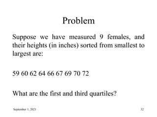
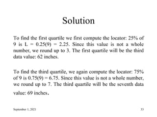
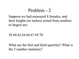
1) List the values in ascending order: 59, 60, 62, 64, 66, 67, 69, 70, 72
2) The number of observations is 9. To find the first quartile (Q1), we take the value at position ⌊(n+1)/4⌋ = ⌊(9+1)/4⌋ = 3.
The third value is 62.
3) To find the third quartile (Q3), we take the value at position ⌊3(n+1)/4⌋ = ⌊3(9+1)/4


![Normalization
Min-max normalization: to [new_minA, new_maxA]
Ex. Let income range $12,000 to $98,000 normalized to [0.0,
1.0]. Then $73,000 is mapped to
Z-score normalization (μ: mean, σ: standard deviation):
Ex. Let μ = 54,000, σ = 16,000. Then
Normalization by decimal scaling
716
.
0
0
)
0
0
.
1
(
000
,
12
000
,
98
000
,
12
600
,
73
A
A
A
A
A
A
min
new
min
new
max
new
min
max
min
v
v _
)
_
_
(
'
A
A
v
v
'
j
v
v
10
' Where j is the smallest integer such that Max(|ν‘|) < 1
225
.
1
000
,
16
000
,
54
600
,
73
](https://image.slidesharecdn.com/3module-2-211213052741/85/3-module-2-59-320.jpg)