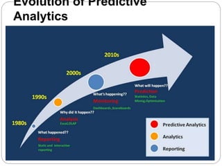
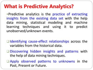
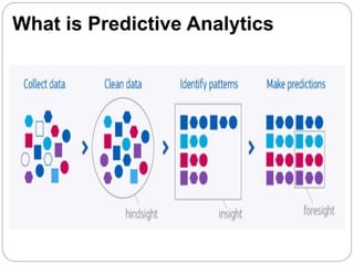
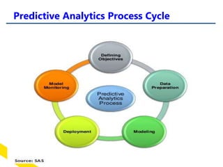
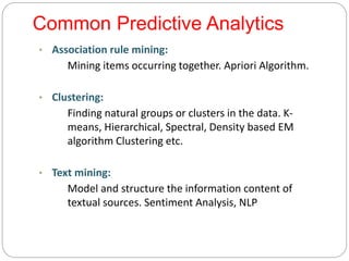
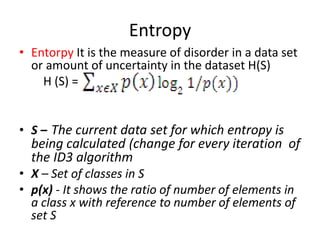
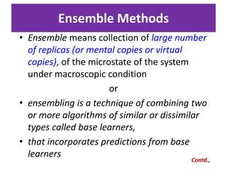
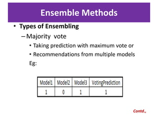
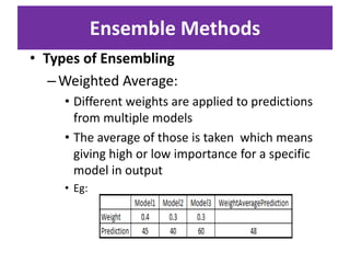
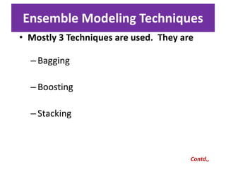
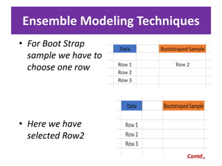
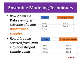
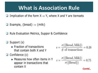
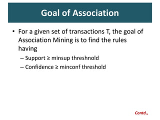
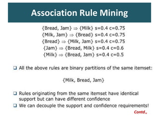
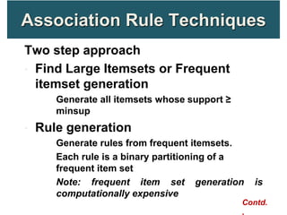
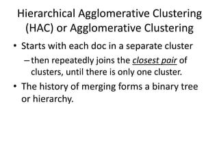
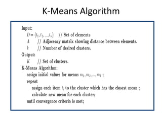
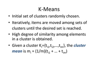
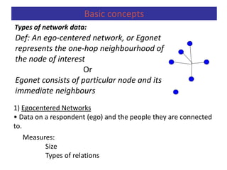
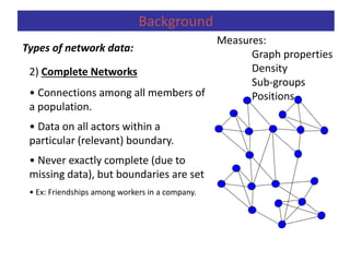
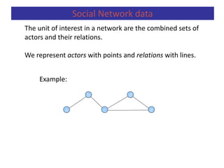
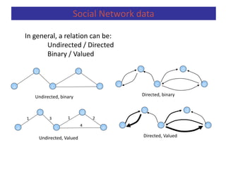
Predictive analytics uses data mining, statistical modeling and machine learning techniques to extract insights from existing data and use them to predict unknown future events. It involves identifying relationships between variables in historical data and applying patterns to unknowns. Predictive analytics is more sophisticated than analytics which has a retrospective focus on understanding trends, while predictive analytics focuses on gaining insights for decision making. Common predictive analytics techniques include regression, classification, time series forecasting, association rule mining and clustering. Ensemble methods like bagging, boosting and stacking combine multiple predictive models to improve performance.

2. Evolution of Predictive
Analytics

3. What is Predictive Analytics?
Predictive analytics is the practice of extracting
insights from the existing data set with the help
data mining, statistical modeling and machine
learning techniques and using it to predict
unobserved/unknown events.
 Identifying cause-effect relationships across the
variables from the historical data.
 Discovering hidden insights and patterns with
the help of data mining techniques.
 Apply observed patterns to unknowns in the
Past, Present or Future.

4. What is Predictive Analytics

5. Predictive Analytics Process Cycle

6. Analytics & Predictive Analytics
 Analytics is the understanding of existing
(retrospective) data with the goal of
understanding trends via comparison
 Developing analytics is the first step towards
deriving predictive analytics
 Predictive Analytics are more sophisticated analytics
that “forward thinking” in nature
 used for gaining insights from mathematical
and/or financial modeling by enhancing
understanding, interpretation and judgment for
the purpose of good decision making

7. © 2011 Predictive Dashboards LLC 7
Comparative Study:: Analytics and Predictive Analytics
Attribute Analytics Predictive Analytics
Purpose:
Understand the Past
Observe Trends
Catalyst for Discussion
Gain Insights
Make Decisions
Take Action
View: Historical and Current Future Oriented
Metrics Type: Lagging Indicators Leading Indicators
Data Used: Raw & Compiled Information
Data Type: Structured Structured and Unstructured
Users: Middle & Senior Mgt
Analysts, End Users
C-Level & Senior Mgt
Strategists, Analysts, Mgrs
Benefits: Gaining an understanding
of data
Productivity Improvements
Gaining Information & Insights
Process Improvements

8. Benefits
Benefits of Analytics:
productivity gains through improved data-
gathering processes
results in less time required for producing
reports and metrics
beneficial Not scalable, not repeatable
Benefits of predictive analytics:
process improvement gains through
improve revenue generation & cost
structures
enhanced decision making
Beneficial, Scalable, repeatable

9. Common Predictive Analytics
• Regression:
 Predicting output variable using its cause-effect
relationship with input variables. OLS Regression, GLM,
Random forests, ANN etc.
• Classification:
Predicting the item class. Decision Tree, Logistic
Regression, ANN, SVM, Naïve Bayes classifier etc.
• Time Series Forecasting:
Predicting future time events given past history. AR,
MA, ARIMA, Triple Exponential Smoothing, Holt-
Winters etc.
Contd.,

10. Common Predictive Analytics
• Association rule mining:
Mining items occurring together. Apriori Algorithm.
• Clustering:
Finding natural groups or clusters in the data. K-
means, Hierarchical, Spectral, Density based EM
algorithm Clustering etc.
• Text mining:
Model and structure the information content of
textual sources. Sentiment Analysis, NLP

11. Regression
 A Regression Model defines three types of
regression models:
 linear,
 Polynomial or Multiple regression
 logistic regression. Or log linear regression

12. Linear Regression
• The simplest form of regression to visualize is
linear regression with a single predictor. A
linear regression technique can be used if the
relationship between x and y can be
approximated with a straight line
Y =  +  X

13. Nonlinear Regression
• the relationship between x and y cannot be
approximated with a straight line. In this case,
a nonlinear regression technique may be used.
Alternatively, the data could be preprocessed
to make the relationship linear.

14. Multivariate Regression
• Multivariate regression refers to regression
with multiple predictors (x1 , x2 , ..., xn). For
purposes of illustration
Y = b0 + b1 X1 + b2 X2.

15. Decision Tree Induction
• A decision tree is a structure that includes a
root node, branches, and leaf nodes.
• Each internal node denotes a test on an
attribute,
• Each branch denotes the outcome of a test,
and
• Each leaf node holds a class label.
• The topmost node in the tree is the root node.

16. Balanced Decision Tree

17. Decision Tree Issues
• Choosing Splitting Attributes
• Ordering of Splitting Attributes
• Splits (No. of Splits to take)
• Tree Structure (few levels are required for a
balanced tree)
• Stopping Criteria
– once training data is perfectly classified tree will stop
– Stopping earlier results overfitting
• Training Data
– Neither too small nor too big
• Pruning – improving of tree is needed by
removing sub-trees when required

18. Entropy
• Entorpy It is the measure of disorder in a data set
or amount of uncertainty in the dataset H(S)
H (S) =
• S – The current data set for which entropy is
being calculated (change for every iteration of
the ID3 algorithm
• X – Set of classes in S
• p(x) - It shows the ratio of number of elements in
a class x with reference to number of elements of
set S

19. Here our Partition is on Colour not on Shapes . After partition we get

20. After partition
24 stars, 25 Diamonds i.e., 24+25 = 49

21. Entropy
• Entropy is calculated for all stars and all
diamonds

22. Entropy

23. Entropy

25. Information Gain
• Information gain is a measure of the decrease
of disorder achieved by partitioning the
original data set

26. CART
• Create Binary Tree
• Uses entropy
• Formula to choose split point, s, for node t:
• PL,PR probability that a tuple in the training set will
be on the left or right side of the tree.

27. CART Example
• At the start, there are six choices for split
point (right branch on equality):
– P(Gender)=2(6/15)(9/15)(2/15 + 4/15 + 3/15)=0.224
– P(1.6) = 0
– P(1.7) = 2(2/15)(13/15)(0 + 8/15 + 3/15) = 0.169
– P(1.8) = 2(5/15)(10/15)(4/15 + 6/15 + 3/15) = 0.385
– P(1.9) = 2(9/15)(6/15)(4/15 + 2/15 + 3/15) = 0.256
– P(2.0) = 2(12/15)(3/15)(4/15 + 8/15 + 3/15) = 0.32
• Split at 1.8

28. What is a Neural Network
• A computer system modeled on the human
brain and nervous system
• NN is usually organized in layers
• Layers are made up of number of inter-
connected nodes
• The connection strengths of neurons are
called weights, that are used to store the
acquired information (training examples)

29. Contd..Neural Networks
• During the learning process the weights are
modified in order to model the particular
learning task correctly on the training
examples.

30. Propagation
Tuple Input
Output
Input

31. CLASSIFICATION
(RULE BASED)

32. Classification Using Rules
• Perform classification using If-Then rules
• Classification Rule: r = <a,c>
Antecedent, Consequent
• May generate from from other techniques
(DT, NN) or generate directly.
• Algorithms: Gen, RX, 1R, PRISM

33. Generating Rules Example

34. CLASSIFICATION TREES
(ENSEMBLED METHODS)

35. Ensemble Methods
• Ensemble means collection of large number
of replicas (or mental copies or virtual
copies), of the microstate of the system
under macroscopic condition
or
• ensembling is a technique of combining two
or more algorithms of similar or dissimilar
types called base learners,
• that incorporates predictions from base
learners
Contd.,

36. • Eg:- A decision of an interviewr depnds on
the feedback of the all the interviewrs in
various rounds
Ensemble Methods

37. • Types of Ensembling:
– 3 types
–Averaging
• Taking the average of predictions from
models in regression
• Predicting of probabilites in classification
problem
Eg:
Ensemble Methods
Contd.,

38. • Types of Ensembling
–Majority vote
• Taking prediction with maximum vote or
• Recommendations from multiple models
Eg:
Ensemble Methods
Contd.,

39. • Types of Ensembling
–Weighted Average:
• Different weights are applied to predictions
from multiple models
• The average of those is taken which means
giving high or low importance for a specific
model in output
• Eg:
Ensemble Methods

40. Ensemble Modeling Techniques
• Mostly 3 Techniques are used. They are
–Bagging
–Boosting
–Stacking
Contd.,

41. Ensemble Modeling Techniques
• Mostly 3 Techniques are used. They are
–Bagging
• Referred as bootstrap aggregation
• BootStrap or Bootstrapping
–It is a sampling technique
–We choose ‘n’ observations from the
original dataset
–The probability of selecting each row
from the dataset is equal for all in each
iteration
Contd.,

42. Ensemble Modeling Techniques
Contd.,
• For Boot Strap
sample we have to
choose one row
• Here we have
selected Row2

43. Ensemble Modeling Techniques
Contd.,
• Row 2 exists in
Data even after
selection of it into
Bootstraped
samples
• Row 1 is again
selected from Data
into Bootstraped
sample again

44. Ensemble Modeling Techniques
Contd.,
• Now Bootstraped samples is ready for
growing trees.
• The above sample use majority vote or
averaging concepts to get final Prediction
• Bagging is mainly used to reduce variance
– Eg: Random Forest

45. Ensemble Modeling Techniques
• Mostly 3 Techniques are used. They are
–Bagging
• Referred as bootstrap aggregation
• BootStrap or Bootstrapping
–It is a sampling technique
–We choose ‘n’ observations from the
original dataset
–The probability of selecting each row
from the dataset is equal for all in each
iteration
Contd.,

46. Ensemble Modeling Techniques
• Mostly 3 Techniques are used. They are
–Boosting
• Avoids overfitting, in which first
algorithm is trained on the entire
dataset.
• Subsequent algorithms are built by
fitting the residuals of first algorithm,
• This gives higher weight for the poor
predicted observations in previous
model to avoid overfitting Contd.,

47. Ensemble Modeling Techniques
–Eg: XGBoost, GBM, ADABOOST, etc.,
• F1(x)=F0(x)+λ0h0(x)=5008.3+0.5∗4991.6=7504.1F1(x)=
F0(x)+λ0h0(x)=5008.3+0.5∗4991.6=7504.1.
• So this person earns $7504.1 per month according to
our model.

48. Ensemble Modeling Techniques
• Third Technique
–Stacking has two layers of machine
learning
Contd.,
• d1,d2,d3 receive
original inputs
feeatres (x)
• Top Layer f() takes the
output of bottom
layers (d1,d2,d3) and
predicts the output
(y)

49. Ensemble Modeling Techniques
• Key Principles for selecting models
– The individual models fulfill particular accuracy
criteria.
– The model predictions of various individual
models are not highly correlated with the
predictions of other models
– Note: This top layer model can also be
replaced by many other simpler formulas like:
• Averaging
• Majority vote
• Weighted Average
Contd.,

50. Ensemble Modeling Techniques
• Advantages
–Proven method of improving accuracy
–Key ingredient for winning almost all the
machine learning hackathons (it is a big
gathering of programmers code in a extreme manner
over a short period of time)
–Make model robust, stable and decent
performance on the test cases
–Ensembling can be used to capture
simple linear or non-linear complex
relationships in data Contd.,

51. Ensemble Modeling Techniques
• Dis-Advantages
–Reduces model interpretability
–Difficult to draw crucial business insights
at the end
–Time consuming activity, not suitable for
real time scenarios
–Selection of ensemble model is difficult
Contd.,

52. Association Rules

53. Association Rules
• Association Rule :
–“finding
–frequent patterns,
–associations,
–correlations, or casual structures
–among sets of items or objects in
transactional/relational databases or any
other informational repository”
– Cross-marketing
– Catalogue Design Contd.,

54. What is Association Rule
– Cross-marketing
– Catalogue Design
• Examples
• {bread}  {milk}
• {soda}  {chips}
• {bread}  {jam}
Given a set of transactions, find rules that will
predict the occurrence of an item based on the
occurrences of other items in the transaction
Contd.,

55. Support and Confidence

56. What is Association Rule
Contd.,

57. Goal of Association
Contd.,
• For a given set of transactions T, the goal of
Association Mining is to find the rules
having
– Support ≥ minsup threshnold
– Confidence ≥ minconf threshold

58. Association Rule Mining
Contd.,

59. Association Rule Techniques
Two step approach
• Find Large Itemsets or Frequent
itemset generation
• Generate all itemsets whose support ≥
minsup
• Rule generation
• Generate rules from frequent itemsets.
• Each rule is a binary partitioning of a
frequent item set
• Note: frequent item set generation is
computationally expensive
Contd.
,

60. Algorithm to Generate ARs
Contd.
,

61. Apriori Algorithm
1. C1 = Itemsets of size one in I;
2. Determine all large itemsets of size 1, L1;
3. i = 1;
4. Repeat
5. i = i + 1;
6. Ci = Apriori-Gen(Li-1);
7. Count Ci to determine Li;
8. until no more large itemsets found;
Contd.
,

62. Working of Apriori Principle
Contd.
,

63. Apriori
Advantages/Disadvantages
 Advantages:
– Uses large itemset property.
– Easily parallelized
– Easy to implement.
 Disadvantages:
– Assumes transaction database is memory
resident.
– Requires up to m database scans.

64. Sequence Rules

65. Sequence Rules
• For a Database D, finding the maximal
sequences among the ‘n’ sequences, that
have certail user-specified minimum
support and confidence

66. Segmentation

67. Segmentation
• For a Database D, finding the maximal
sequences among the ‘n’ sequences, that
have certail user-specified minimum
support and confidence

68. Clustering Approaches
Sampling Compression
Clustering
Hierarchical Partitional Categorical Large DB
Agglomerative Divisive

69. Types of Clustering
• Hierarchical – Nested set of clusters created.
• Partitional – One set of clusters created.
• Incremental – Each element handled one at a
time.
• Simultaneous – All elements handled
together.
• Overlapping/Non-overlapping

70. Hierarchical Clustering
• Build a tree-based hierarchical taxonomy
(dendrogram) from a set of unlabeled examples
• Recursive application of a standard clustering
algorithm can produce a hierarchical clustering
animal
vertebrate
fish reptile amphib. mammal worm insect crustacean
invertebrate

71. Hierarchical Clustering
• Agglomerative
– Bottom up approach
– Start with single-instance clusters
– At each step join the two closest clusters
– Design Decision: distance between clusters
• Eg: two closest instances in clusters vs distance
between means
• Divisive / deglomarative
– Top Down Approach
– Start with one universal cluster
– Find two clusters
– Proceed recursively on each subset
– Can be very fast
Both produce a Dendrogram
Top Down
Approach
Bottom up
Approach

72. Hierarchical Agglomerative Clustering
(HAC) or Agglomerative Clustering
• Starts with each doc in a separate cluster
–then repeatedly joins the closest pair of
clusters, until there is only one cluster.
• The history of merging forms a binary tree
or hierarchy.

73. K-Means Algorithm

74. K – Means Clustering
Now group this data into two clusters

75. K – Means Clustering
• Randomly initialize
two points called
centroids

76. • Colour the datasets
in red and blue
• Find the nearest
dataset for Red or
Blue coloured
centroid
• Move the centroids
K – Means Clustering

77. • After calculating
the mean of all
centroids for both
the colour i.e.,
Red and Blue
• Closest to the
both the colours
K – Means Clustering

78. K-means clustering
• Calculate the
average of blue
points and red
points and move
the centroid again

79. K-means Clustering
• Calculate the
average and mean
of blue and red
points then move
the centroid again
• Continue this steps
of iteration
• At a particular point
cluster centroids
will not change

80. K-Means
• Initial set of clusters randomly chosen.
• Iteratively, items are moved among sets of
clusters until the desired set is reached.
• High degree of similarity among elements
in a cluster is obtained.
• Given a cluster Ki={ti1,ti2,…,tim}, the cluster
mean is mi = (1/m)(ti1 + … + tim)

81. Social Network Analysis
(SNA)

82. Social network analysis is:
• a set of relational methods for systematically
understanding and identifying connections among actors
Introduction

83. • Actors (nodes, points, vertices):
- Individuals, Organizations, Events …
• Relations (lines, arcs, edges, ties): between pairs of actors.
- Undirected (symmetric) / Directed (asymmetric)
- Binary / Valued
Basic concepts
Network Components

84. 1) Egocentered Networks
• Data on a respondent (ego) and the people they are connected
to.
Measures:
Size
Types of relations
Basic concepts
Types of network data:
Def: An ego-centered network, or Egonet
represents the one-hop neighbourhood of
the node of interest
Or
Egonet consists of particular node and its
immediate neighbours

85. 2) Complete Networks
• Connections among all members of
a population.
• Data on all actors within a
particular (relevant) boundary.
• Never exactly complete (due to
missing data), but boundaries are set
• Ex: Friendships among workers in a company.
Measures:
Graph properties
Density
Sub-groups
Positions
Background
Types of network data:

86. The unit of interest in a network are the combined sets of
actors and their relations.
We represent actors with points and relations with lines.
Example:
Social Network data
a
b
c e
d

87. In general, a relation can be:
Undirected / Directed
Binary / Valued
a
b
c e
d
Undirected, binary Directed, binary
a
b
c e
d
a
b
c e
d
Undirected, Valued Directed, Valued
a
b
c e
d
1 3
4
21
Social Network data

88. From pictures to matrices
Undirected, binary Directed, binary
a b c d e
a
b
c
d
e
1
1
1 1 1
1 1
a b c d e
a
b
c
d
e
1
1 1
1 1 1
1 1
1 1
Basic Data Structures
Social Network data
a
b
c e
d
a
b
c e
d

89. d e
c
Indirect connections are what make networks
systems. One actor can reach another if there is
a path in the graph connecting them.
a
b
c e
d
f
b f
a
Connectivity
Measuring Networks

90. Distance is measured by the (weighted) number of
relations separating a pair, Using the shortest path.
Actor “a” is:
1 step from 4
2 steps from 5
3 steps from 4
4 steps from 3
5 steps from 1
Distance & number of paths
Measuring Networks
a

91. An information
network:
Email exchanges
within the
Reagan white
house, early
1980s
(source: Blanton,
1995)
Measuring Networks

92. Centrality refers to (one dimension of) location, identifying
where an actor resides in a network.
Centrality
Measuring Networks
Centrality is fairly straight forward: we want to
identify which nodes are in the ‘center’ of the
network. In the sense that they have many and
important connections.
Three standard centrality measures capture a wide
range of “importance” in a network:
Degree
Closeness
Betweenness

93. The most intuitive notion of centrality focuses on
degree. Degree is the number of lines, and the
actor with the most lines is the most important:
Centrality
Measuring Networks

94. Centrality
Measuring Networks
Relative measure of Degree Centrality:
1
),(
)(' 1


 
n
ppa
PC
ki
n
i
kD
Degree Centrality:
),()(
1
ki
n
i
kD ppaPC



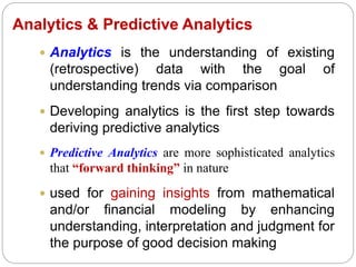
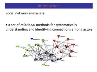
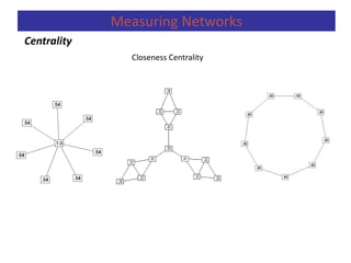
95. A second measure is closeness centrality. An actor
is considered important if he/she is relatively close to all
other actors.
Closeness is based on the inverse of the
distance of each actor to every other actor in the
network.
Closeness Centrality:
Relative Closeness Centrality
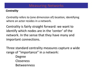
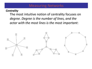
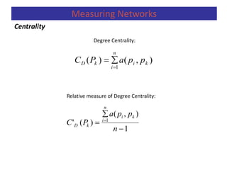
Centrality
Measuring Networks
1
1
)],([)( 

 ki
n
i
kC ppdPC
),(
1
1
),(
)('
1
1
1
ki
n
i
ki
n
i
kC
ppd
n
n
ppd
PC




















96. Closeness Centrality
Centrality
Measuring Networks

97. Betweenness Centrality:
Model based on communication flow: A person who lies
on communication paths can control communication flow, and is
thus important. Betweenness centrality counts the number of
shortest paths between i and k that actor j resides on.
b
a
C d e f g h
Centrality
Measuring Networks

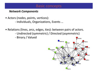
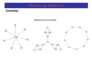
98. Centrality
Measuring Networks
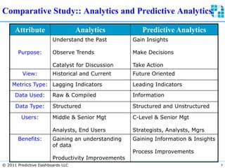
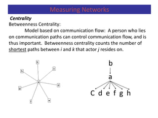
Betweenness centrality can be defined in terms of probability (1/gij),
CB(pk) = iij(pk) = =
gij = number of geodesics that bond actors pi and pj.
gij(pk)= number of geodesics which bond pi and pj and content pk.
iij(pk) = probability that actor pk is in a geodesic randomly chosen among the
ones which join pi and pj.
Betweenness centrality is the sum of these probabilities (Freeman, 1979).
)(*
g
1
ij
kij pg
ij
kij
g
)(pg
Normalizad: C’B(pk) = CB(pk) / [(n-1)(n-2)/2]

99. Betweenness Centrality:
Centrality
Measuring Networks

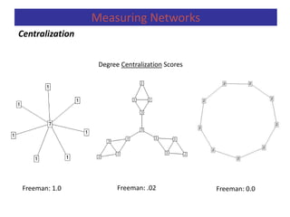
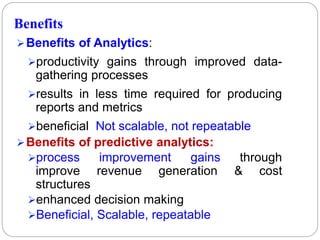
100. If we want to measure the degree to which the graph as a whole is centralized, we look
at the dispersion of centrality:
Freeman’s general formula for centralization (which ranges from 0 to 1):
 
)]2)(1[(
)()(1
*




nn
pCpC
C
n
i iDD
D
Centralization
Measuring Networks

101. Degree Centralization Scores
Freeman: 1.0 Freeman: .02 Freeman: 0.0
Centralization
Measuring Networks

102. Density
Measuring Networks
The more actors are connected to one another, the more dense the network will
be.
Undirected network: n(n-1)/2 = 2n-1 possible pairs of actors.
Δ =
Directed network: n(n-1)*2/2 = 2n-2possible lines.
ΔD =
2/)1( nn
L
)1( nn
L

103. Freeman: .25 Freeman: .23 Freeman: 0.25
Density
Measuring Networks

104. UCINET
•The Standard network analysis program, runs in Windows
•Good for computing measures of network topography for single
nets
•Input-Output of data is a special 2-file format, but is now able to
read PAJEK files directly.
•Not optimal for large networks
•Available from:
Analytic Technologies
Social Network Software

105. PAJEK
•Program for analyzing and plotting very large networks
•Intuitive windows interface
•Started mainly a graphics program, but has expanded to a wide range of
analytic capabilities
•Can link to the R statistical package
•Free
•Available from: http://vlado.fmf.uni-lj.si/pub/networks/pajek/
Social Network Software

106. NetDraw
•Also very new, but by one of the best known names in
network analysis software.
•Free
Social Network Software