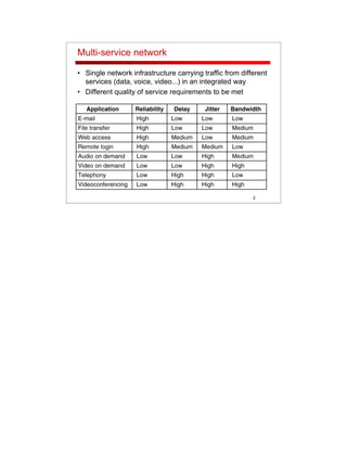
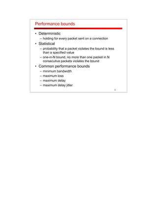
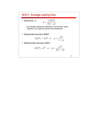
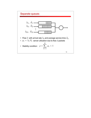
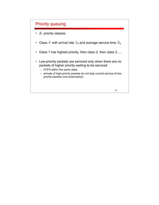
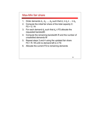
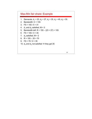
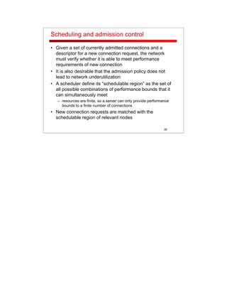
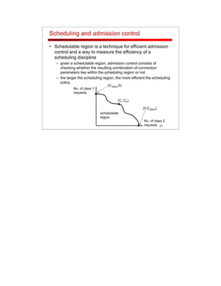
Packet Scheduling
for QoS management
TELCOM2321 – CS2520
Wide Area Networks
Dr. Walter Cerroni
University of Bologna – Italy
Visiting Assistant Professor at SIS, Telecom Program
Slides partly based on Dr. Znati’s material
2
Multi-service network
• Single network infrastructure carrying traffic from different
services (data, voice, video...) in an integrated way
• Different quality of service requirements to be met
3
Performance bounds
• Deterministic
– holding for every packet sent on a connection
• Statistical
– probability that a packet violates the bound is less
than a specified value
– one-in-N bound, no more than one packet in N
consecutive packets violates the bound
• Common performance bounds
– minimum bandwidth
– maximum loss
– maximum delay
– maximum delay jitter
4
Performance bounds: Delay jitter
• Delay jitter bound requires that the network limit
the difference between the largest and the
smallest delays experienced by packets
delayprob.densityfunction
delay
propagation
delay
jitter
average
delay
worst-case
delay
5
Performance bounds: Delay jitter
• Delay jitter bound is useful for audio/video playback,
where receiver can compensate delay variations
– delaying the first packet by the delay-jitter bound in an elasticity
buffer
– playing back packets at a constant rate from the buffer
Time
CBR playback
at the client
playback
buffer delay
variable
network delay
CBR streaming
at the source
Cumulativedata
reception
at the client
buffered
data
6
Performance bounds: Delay jitter
• Playback buffer delay must be appropriate
– if too short, it will cause losses
– if too large, it will affect interactivity
Time
Cumulativedata
loss
too large e2e delay
7
The role of the network
• The network should have enough resources
available to be able to satisfy the performance
bounds required by the application
– admission control
– congestion control
• The network should efficiently manage the
resources available in order to guarantee a
quality of service acceptable to the application
– packet scheduling at intermediate nodes
8
Packet scheduling
• Packets are queued at intermediate nodes
– store and forward
• The server on each queue must
– decide which packet to service next
– manage the queue of backlogged packets
• The server uses a scheduling discipline to
– fairly share the resources
– provide performance guarantees
• Trade-off between
– traffic isolation
• circuit switching: guaranteed dedicated resources
– resource sharing
• packet switching: complete resource sharing
9
Scheduling policy requirements
• A scheduler should be
– not too expensive in terms of required hardware
– scalable
• the number of operations to implement a discipline should be
as independent as possible of the number of scheduled
connections
– fair
• it should allocate a fair share of the link capacity and output
queue buffer to each connection
– protective
• the misbehavior of one source should not affect the
performance received by other sources
10
The simplest scheduler: FCFS or FIFO
• First Come First Served or First In First Out
• Packets are served in the same order as they arrive
• Most commonly used scheduling discipline
• Example
– M/G/1 queue: Poisson arrivals, generic service time
• Stability condition on server utilization
• Probability of idle server state
queue server
arrival rate departure rate
average
service time
11
M/G/1: Average waiting time
• Each packet arriving at the queue
– is served immediately, if server is idle
• waiting time = 0 with probability
– must wait for the packet currently being served to finish its
service, if server is busy
• waiting time = residual service time with prob.
• average residual service time:
– must wait also for all packets previously queued to finish their
service, if queue is not empty
• waiting time = sum of service times for each queued packet
• average number of packets in the queue (Little’s theorem):
• Average waiting time
12
M/G/1: Average waiting time
• Solving for :
– the average waiting time depends on arrival rate, server
utilization (i.e. load) and service time distribution
• Exponential services: M/M/1
• Deterministic services: M/D/1
13
Limitations of FCFS
• All packets are serviced the same way
• No consideration for delay sensitivity
– small packets must wait for long packets to be serviced
• Unfair
– connections with large packets usually receive better services by
getting higher percentage of server time
• Not protective
– greedy connections are advantaged over friendlier connections
– an excessively active connection may cause other connections
implementing congestion control to back off more than required
• The cause is complete resource sharing without traffic
isolation
– isolation through separate queues for different traffic flows or
classes sharing the same bandwidth
14
Separate queues
• Flow with arrival rate and average service time
• server utilization due to flow packets
• Stability condition:
...
15
Priority queuing
• priority classes
• Class with arrival rate and average service time
• Class 1 has highest priority, then class 2, then class 3, ...
• Low-priority packets are serviced only when there are no
packets of higher priority waiting to be serviced
– FCFS within the same class
– arrivals of high-priority packets do not stop current service of low-
priority packets (non-preemptive)
16
M/G/1 with priorities: Average waiting time
• Each class packet arriving at the queue
– is served immediately, if server is idle
• waiting time = 0 with probability
– must wait for the packet currently being served to finish its
service, if server is busy
• average residual service time:
– must wait for all packets of class previously queued to
finish their service
• average number of class packets in the queue:
each requiring average service time
– must wait also for all packets of class that have been
received during its waiting time to finish their service
• average number of class packets arrived during class packet
waiting time:
each requiring average service time
17
M/G/1 with priorities: Average waiting time
• Average class waiting time
• Solving for
• Same expression in recursive format (Cobham’s formula)
18
Example: 2 classes
Assuming identical exponential services for both classes and
we get
19
Example: 2 classes
0
2
4
6
8
10
12
14
16
18
20
0 0.2 0.4 0.6 0.8 1
no priorities
20
Limitations of priority queuing
• Effective only when high priority traffic is a small part of
the total traffic
– efficient admission control and policing may be required
• Not protective
– a misbehaving source at a higher priority level can increase delay
at lower priority levels
• Unfair
– starvation of low-priority queues in case of heavy high-priority
traffic
• More sophisticated scheduling disciplines are required
– better traffic isolation
– fairer resource sharing
21
Conservation Law
• Traffic isolation while sharing resources is limited by the
conservation law
• The sum of the mean queuing delays received by the set
of multiplexed connections, weighted by their share of the
link's load, is independent of the scheduling discipline
• In other words, a scheduling discipline can reduce a
particular connection's mean delay, compared with
FCFS, only at the expense of another connection
• Valid if server is idle only when queues are empty
– work-conserving schedulers
22
Non-Work Conserving Schedulers
• A non-work conserving scheduler may idle even when
packets are currently waiting for service
• A non-work conserving scheduler can reduce delay jitter
if packets are only serviced at their eligibility times
– packets are serviced no faster than the allowed rate
– in case of exceeding bursts, non-eligible packets are retained
– introducing idle time makes the traffic more predictable
– bursts do not build up within the network
• A(k), arrival time for k-th packet
• E(k), eligibility time for k-th packet
• XMIN, inverse of the highest allowed packet rate
• E(k+1) = max { E(k) + XMIN, A(k+1) }
• Bandwidth wasted during forced idle times
• Jitter reduced at the cost of increased average delay
23
Max-Min fair share
• Resources should be shared in a fair way, especially
when they are not sufficient to satisfy all requests
• Max-Min fair share
– bandwidth allocation technique that tries to maximize the
minimum share for non-satisfied flows
• Basic principles
– resources are allocated in order of increasing demands
– users with relatively small demands are satisfied
– no user gets a resource share larger than its demand
– users with unsatisfied demands get an equal share of unused
resources
24
Max-Min fair share
1. Order demands d1, d2, ..., dN such that d1 ≤ d2 ≤ ... ≤ dN
2. Compute the initial fair share of the total capacity C:
FS = C / N
3. For each demand dk such that dk ≤ FS allocate the
requested bandwidth
4. Compute the remaining bandwidth R and the number of
unsatisfied demands M
5. Repeat steps 3 and 4 using the updated fair share
FS = R / M until no demand left is ≤ FS
6. Allocate the current FS to remaining demands
25
Max-Min fair share: Example
1. Demands: d1 = 23, d2 = 27, d3 = 35, d4 = 45, d5 = 55
2. Bandwidth: C = 155
3. FS = 155 / 5 = 31
4. d1 and d2 satisfied, M = 3
5. Bandwidth left: R = 155 – (23 + 27) = 105
6. FS = 105 / 3 = 35
7. d3 satisfied, M = 2
8. R = 105 – 35 = 70
9. FS = 70 / 2 = 35
10. d4 and d5 not satisfied they get 35
26
Scheduling and admission control
• Given a set of currently admitted connections and a
descriptor for a new connection request, the network
must verify whether it is able to meet performance
requirements of new connection
• It is also desirable that the admission policy does not
lead to network underutilization
• A scheduler define its “schedulable region” as the set of
all possible combinations of performance bounds that it
can simultaneously meet
– resources are finite, so a server can only provide performance
bounds to a finite number of connections
• New connection requests are matched with the
schedulable region of relevant nodes
27
Scheduling and admission control
• Schedulable region is a technique for efficient admission
control and a way to measure the efficiency of a
scheduling discipline
– given a schedulable region, admission control consists of
checking whether the resulting combination of connection
parameters lies within the scheduling region or not
– the larger the scheduling region, the more efficient the scheduling
policy
No. of class 1
requests
No. of class 2
requests
(C1,C2)
(C1MAX,0)
schedulable
region
(0,C2MAX)

Packet scheduling

  • 1.
    Packet Scheduling for QoSmanagement TELCOM2321 – CS2520 Wide Area Networks Dr. Walter Cerroni University of Bologna – Italy Visiting Assistant Professor at SIS, Telecom Program Slides partly based on Dr. Znati’s material
  • 2.
    2 Multi-service network • Singlenetwork infrastructure carrying traffic from different services (data, voice, video...) in an integrated way • Different quality of service requirements to be met
  • 3.
    3 Performance bounds • Deterministic –holding for every packet sent on a connection • Statistical – probability that a packet violates the bound is less than a specified value – one-in-N bound, no more than one packet in N consecutive packets violates the bound • Common performance bounds – minimum bandwidth – maximum loss – maximum delay – maximum delay jitter
  • 4.
    4 Performance bounds: Delayjitter • Delay jitter bound requires that the network limit the difference between the largest and the smallest delays experienced by packets delayprob.densityfunction delay propagation delay jitter average delay worst-case delay
  • 5.
    5 Performance bounds: Delayjitter • Delay jitter bound is useful for audio/video playback, where receiver can compensate delay variations – delaying the first packet by the delay-jitter bound in an elasticity buffer – playing back packets at a constant rate from the buffer Time CBR playback at the client playback buffer delay variable network delay CBR streaming at the source Cumulativedata reception at the client buffered data
  • 6.
    6 Performance bounds: Delayjitter • Playback buffer delay must be appropriate – if too short, it will cause losses – if too large, it will affect interactivity Time Cumulativedata loss too large e2e delay
  • 7.
    7 The role ofthe network • The network should have enough resources available to be able to satisfy the performance bounds required by the application – admission control – congestion control • The network should efficiently manage the resources available in order to guarantee a quality of service acceptable to the application – packet scheduling at intermediate nodes
  • 8.
    8 Packet scheduling • Packetsare queued at intermediate nodes – store and forward • The server on each queue must – decide which packet to service next – manage the queue of backlogged packets • The server uses a scheduling discipline to – fairly share the resources – provide performance guarantees • Trade-off between – traffic isolation • circuit switching: guaranteed dedicated resources – resource sharing • packet switching: complete resource sharing
  • 9.
    9 Scheduling policy requirements •A scheduler should be – not too expensive in terms of required hardware – scalable • the number of operations to implement a discipline should be as independent as possible of the number of scheduled connections – fair • it should allocate a fair share of the link capacity and output queue buffer to each connection – protective • the misbehavior of one source should not affect the performance received by other sources
  • 10.
    10 The simplest scheduler:FCFS or FIFO • First Come First Served or First In First Out • Packets are served in the same order as they arrive • Most commonly used scheduling discipline • Example – M/G/1 queue: Poisson arrivals, generic service time • Stability condition on server utilization • Probability of idle server state queue server arrival rate departure rate average service time
  • 11.
    11 M/G/1: Average waitingtime • Each packet arriving at the queue – is served immediately, if server is idle • waiting time = 0 with probability – must wait for the packet currently being served to finish its service, if server is busy • waiting time = residual service time with prob. • average residual service time: – must wait also for all packets previously queued to finish their service, if queue is not empty • waiting time = sum of service times for each queued packet • average number of packets in the queue (Little’s theorem): • Average waiting time
  • 12.
    12 M/G/1: Average waitingtime • Solving for : – the average waiting time depends on arrival rate, server utilization (i.e. load) and service time distribution • Exponential services: M/M/1 • Deterministic services: M/D/1
  • 13.
    13 Limitations of FCFS •All packets are serviced the same way • No consideration for delay sensitivity – small packets must wait for long packets to be serviced • Unfair – connections with large packets usually receive better services by getting higher percentage of server time • Not protective – greedy connections are advantaged over friendlier connections – an excessively active connection may cause other connections implementing congestion control to back off more than required • The cause is complete resource sharing without traffic isolation – isolation through separate queues for different traffic flows or classes sharing the same bandwidth
  • 14.
    14 Separate queues • Flowwith arrival rate and average service time • server utilization due to flow packets • Stability condition: ...
  • 15.
    15 Priority queuing • priorityclasses • Class with arrival rate and average service time • Class 1 has highest priority, then class 2, then class 3, ... • Low-priority packets are serviced only when there are no packets of higher priority waiting to be serviced – FCFS within the same class – arrivals of high-priority packets do not stop current service of low- priority packets (non-preemptive)
  • 16.
    16 M/G/1 with priorities:Average waiting time • Each class packet arriving at the queue – is served immediately, if server is idle • waiting time = 0 with probability – must wait for the packet currently being served to finish its service, if server is busy • average residual service time: – must wait for all packets of class previously queued to finish their service • average number of class packets in the queue: each requiring average service time – must wait also for all packets of class that have been received during its waiting time to finish their service • average number of class packets arrived during class packet waiting time: each requiring average service time
  • 17.
    17 M/G/1 with priorities:Average waiting time • Average class waiting time • Solving for • Same expression in recursive format (Cobham’s formula)
  • 18.
    18 Example: 2 classes Assumingidentical exponential services for both classes and we get
  • 19.
  • 20.
    20 Limitations of priorityqueuing • Effective only when high priority traffic is a small part of the total traffic – efficient admission control and policing may be required • Not protective – a misbehaving source at a higher priority level can increase delay at lower priority levels • Unfair – starvation of low-priority queues in case of heavy high-priority traffic • More sophisticated scheduling disciplines are required – better traffic isolation – fairer resource sharing
  • 21.
    21 Conservation Law • Trafficisolation while sharing resources is limited by the conservation law • The sum of the mean queuing delays received by the set of multiplexed connections, weighted by their share of the link's load, is independent of the scheduling discipline • In other words, a scheduling discipline can reduce a particular connection's mean delay, compared with FCFS, only at the expense of another connection • Valid if server is idle only when queues are empty – work-conserving schedulers
  • 22.
    22 Non-Work Conserving Schedulers •A non-work conserving scheduler may idle even when packets are currently waiting for service • A non-work conserving scheduler can reduce delay jitter if packets are only serviced at their eligibility times – packets are serviced no faster than the allowed rate – in case of exceeding bursts, non-eligible packets are retained – introducing idle time makes the traffic more predictable – bursts do not build up within the network • A(k), arrival time for k-th packet • E(k), eligibility time for k-th packet • XMIN, inverse of the highest allowed packet rate • E(k+1) = max { E(k) + XMIN, A(k+1) } • Bandwidth wasted during forced idle times • Jitter reduced at the cost of increased average delay
  • 23.
    23 Max-Min fair share •Resources should be shared in a fair way, especially when they are not sufficient to satisfy all requests • Max-Min fair share – bandwidth allocation technique that tries to maximize the minimum share for non-satisfied flows • Basic principles – resources are allocated in order of increasing demands – users with relatively small demands are satisfied – no user gets a resource share larger than its demand – users with unsatisfied demands get an equal share of unused resources
  • 24.
    24 Max-Min fair share 1.Order demands d1, d2, ..., dN such that d1 ≤ d2 ≤ ... ≤ dN 2. Compute the initial fair share of the total capacity C: FS = C / N 3. For each demand dk such that dk ≤ FS allocate the requested bandwidth 4. Compute the remaining bandwidth R and the number of unsatisfied demands M 5. Repeat steps 3 and 4 using the updated fair share FS = R / M until no demand left is ≤ FS 6. Allocate the current FS to remaining demands
  • 25.
    25 Max-Min fair share:Example 1. Demands: d1 = 23, d2 = 27, d3 = 35, d4 = 45, d5 = 55 2. Bandwidth: C = 155 3. FS = 155 / 5 = 31 4. d1 and d2 satisfied, M = 3 5. Bandwidth left: R = 155 – (23 + 27) = 105 6. FS = 105 / 3 = 35 7. d3 satisfied, M = 2 8. R = 105 – 35 = 70 9. FS = 70 / 2 = 35 10. d4 and d5 not satisfied they get 35
  • 26.
    26 Scheduling and admissioncontrol • Given a set of currently admitted connections and a descriptor for a new connection request, the network must verify whether it is able to meet performance requirements of new connection • It is also desirable that the admission policy does not lead to network underutilization • A scheduler define its “schedulable region” as the set of all possible combinations of performance bounds that it can simultaneously meet – resources are finite, so a server can only provide performance bounds to a finite number of connections • New connection requests are matched with the schedulable region of relevant nodes
  • 27.
    27 Scheduling and admissioncontrol • Schedulable region is a technique for efficient admission control and a way to measure the efficiency of a scheduling discipline – given a schedulable region, admission control consists of checking whether the resulting combination of connection parameters lies within the scheduling region or not – the larger the scheduling region, the more efficient the scheduling policy No. of class 1 requests No. of class 2 requests (C1,C2) (C1MAX,0) schedulable region (0,C2MAX)