Operations Research MBA Notes .pdf

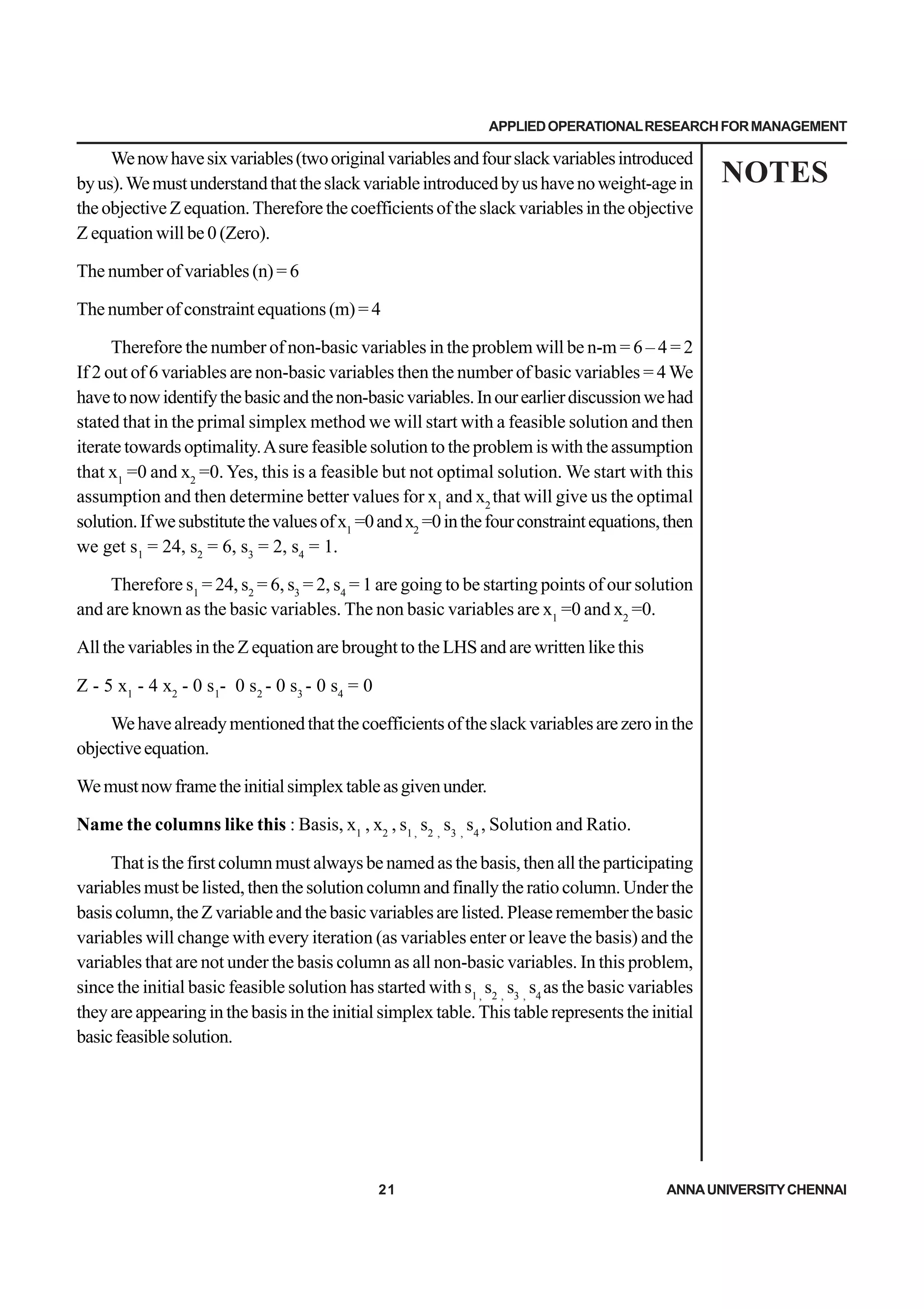
MBA
(DISTANCE MODE)
DBA 1701
APPLIED OPERATIONAL RESEARCH
FOR MANAGEMENT
III SEMESTER
COURSE MATERIAL
Centre for Distance Education
Anna University Chennai
Chennai – 600 025

ii
Author
Mr
Mr
Mr
Mr
Mr. N
. N
. N
. N
. N. Senthil K
. Senthil K
. Senthil K
. Senthil K
. Senthil Kumar
umar
umar
umar
umar,
,
,
,
,
Lecturer,
Department of Management Studies,
Anna University Chennai,
Chennai - 600 025.
Dr
Dr
Dr
Dr
Dr.T
.T
.T
.T
.T.V
.V
.V
.V
.V.Geetha
.Geetha
.Geetha
.Geetha
.Geetha
Professor
Department of Computer Science and Engineering
Chennai - 600 025
Dr
Dr
Dr
Dr
Dr.H.P
.H.P
.H.P
.H.P
.H.Peer
eer
eer
eer
eeru Mohamed
u Mohamed
u Mohamed
u Mohamed
u Mohamed
Professor
Department of Management Studies
Chennai - 600 025
Dr
Dr
Dr
Dr
Dr.C
.C
.C
.C
.C. Chella
. Chella
. Chella
. Chella
. Chellappan
ppan
ppan
ppan
ppan
Professor
Chennai - 600 025
Dr
Dr
Dr
Dr
Dr.A.K
.A.K
.A.K
.A.K
.A.Kannan
annan
annan
annan
annan
Professor
Chennai - 600 025
Copyrights Reserved
(For Private Circulation only)
Editorial Board
Reviewer
Mr
Mr
Mr
Mr
Mr.Ja
.Ja
.Ja
.Ja
.Jay
y
y
y
yanth Jacob
anth Jacob
anth Jacob
anth Jacob
anth Jacob
Senior Lecturer,
Department of Management Studies,
Anna University Chennai,
Chennai - 25

ACKNOWLEDGEMENT
The author has drawn inputs from several sources for the preparation of this course material, to meet the
requirementsofthesyllabus.Theauthorgratefullyacknowledgesthefollowingsources:
• Pannerselvam R, Operations Research, Prentice Hall of India, New Delhi.
• HamdyA. Taha, Operations Research –An Introduction, Sixth Edition, Prentice Hall of India, New
Delhi.
• GuptaP.KandManMohan,ProblemsinOperationsResearch(Methods&Solutions),SultanChand&
Sons, New Delhi.
• Kalavathy.S.OperationsResearch,VikasPublishingHousePvt.Ltd
Inspite of at most care taken to prepare the list of references any omission in the list is only accidental and
notpurposeful.
Mr.Jayanth Jacob
Author
v

DBA 1701 APPLIED OPERATIONAL RESEARCH FOR MANAGEMENT
UNIT I – INTRODUCTION TO LINEAR PROGRAMMING (LP)
Introduction to applications of operations research in functional areas of management. Linear programming-
Formulation, Solution by graphical and simplex methods (primal –penalty, two phase), Special cases, Dual
simplexmethod,Principlesofduality,Sensitivityanalysis.
UNIT II – LINEAR PROGRAMMING EXTENSIONS
Transportationmodels(minimizingandmaximizingcases)–Balancedandunbalancedcases–Initialbasicfeasible
solution by N-W corner rule, least cost and Vogel’s approximation methods. Check for optimality. Solution by
MODI /Stepping stone method. Cases of degeneracy. Transhipment models.
UNIT III – INTEGER LINEAR PROGRAMMINGAND GAME THEORY
Solution to pure and mixed integer programming problem by Branch and bound and cutting plane algorithms.
Gametheory-Twopersonzerosumgames-saddlepoint,DominanceRule,ConvexLinearcombination(averages),
methodsofmatrices,graphicalandLPsolutions.
UNIT IV – DYNAMIC PROGRAMMING, SIMULATIONAND DECISION THEORY
Dynamicprogramming(DP)–Deterministiccases–Maximizingandminimizingproblems.DPtechniquesforLP
problems. Decision making under risk – Decision trees – Decision making under uncertainty.Application of
simulationtechniquesfordecisionmaking.
UNIT V – QUEUINGTHEORYAND REPLACEMENT MODELS
Queuing theory – single and multi-channel models – Infinite number of customers and infinite calling source.
Replacementmodels–Individualreplacementmodels(withandwithouttimevalueofmoney)–Groupreplacement
models.
REFERENCES
1. Paneerselvam R., Operations Research, Prentice Hall of India, Fourth print,August 2003.
2. TulsianP.C,VishalPandey,QuantitativeTechniques(Theoryandproblems),PearsonEducation(Asia),
First Indian Reprint, 2002
vii

CONTENTS
UNIT I
INTRODUCTION TO LINEAR
PROGRAMMING (LP)
1.1 FORMULATION OF LINEAR PROGRAMMING PROBLEM (LPP) 3
1.2 SOLUTION TO LPP THOUGHT GRA[HICAL METHOD 8
1.3 INTRODUCTION TO SOLUTIONS TO LPP THROUGH
SIMPLEX METHOD. 18
1.3.1 Primal Simplex Method 19
1.3.2 Big-M or Penalty Method. 32
1.3.3 Two-Phase Method. 36
1.3.4 Dual Simplex Method 41
1.4 PRINCIPLE OF DUALITY 46
1.5 SENSITIVITYANALYSIS 48
UNIT II
LINEAR PROGRAMMING EXTENSIONS
2.1 TRANSPORTATION MODELS 57
2.1.1 MinimisingProblems 57
2.1.2 MaximisingProblems 74
2.1.3 Transhipment Models 79
UNIT III
INTEGER LINEAR PROGRAMMINGAND
GAMETHEORY
3. 1 INTEGER PROGRAMMING 87
3.1.1 Graphical Method 88
3.1.2 Gomory’s Cutting Plane Method 95
3.2 GAMETHEORY 101
ix

3.2.1 Solution through saddle point 102
3.2.2 Solution through rule of dominance 104
3.2.3 Solution by Oddment method 106
3.2.4 Solution by Graphical method 107
3.2.5 Solution by method of matrices 112
3.2.6 Solution by method of convex linear combinations 114
3.2.7 Solution by LPP 119
UNIT IV
DYNAMIC PROGRAMMING, SIMULATIONAND
DECISION THEORY
4.1 DYNAMIC PROGRAMMING 127
4.2 SIMULATION 133
4.3 DECISION THEORY 139
UNIT V
QUEUINGTHEORYAND REPLACEMENT
MODELS
5.1 QUEUINGTHEORY 153
5.1.1 Single Channel Models 156
5.1.2 Multi Channel Models 158
5.2 REPLACEMENTMODELS 162
5.2.1 Replacement of Items that deteriorate with time (Capital Items) 162
5.2.2 Replacement of Items that fail suddenly (Group Replacement) 169
x

APPLIEDOPERATIONALRESEARCHFORMANAGEMENT
NOTES
1 ANNAUNIVERSITYCHENNAI
UNIT I
INTRODUCTION TO LINEAR
PROGRAMMING (LP)
INTRODUCTION
Operations Research (OR) (a term coined by McClosky and Trefthen in 1940) was
atechniquethatevolvedduringWorldWarIItoeffectivelyusethelimitedmilitaryresources
and yet achieve the best possible results in military operations. In essence you can state
that OR is a technique that helps achieve best (optimum) results under the given set of
limited resources. Over the years, OR has been adapted and used very much in the
manufacturingsectortowardsoptimizationofresources.Thatistouseminimumresources
toachievemaximumoutputorprofitorrevenue.
Learning Objectives
Thelearningobjectivesinthisunitare
1. ToformulateaLinearprogrammingproblem(LPP)fromsetofstatements.
2. To solve the LPPusing graphical method ( For 2 variables)
3. To solve the LPP using primal simplex method ( For > 2 variables and all <=
constraints)
4. TosolvetheLPPusingBig-MandTwo-Phasemethods(For>2variablesandall
mixedconstraints)
5. TosolvetheLPPusingdualsimplexmethod(For>2variablesandthesolutionis
infeasible)
6. We also have a look at the effect of changing the values of parameters on the
decisionvariables(SensitivityAnalysis)
Applications of Operations Research in functional areas of Management
The models of OR can be used by economists, statisticians, administrators and
techniciansbothindefenceandinbusiness.IngeneralORcanbeappliedinallthefunctional
areasofManagementnamely.,Accounting,Construction,FacilitiesPlanning,Marketing,
Finance, Personnel, Research and Development and Production.

DBA 1701
NOTES
Accounting
Assigningauditteamseffectively
Creditpolicyanalysis
CashflowplanningDevelopingstandardcosts
Establishingcostsforbyproducts
Planningofdelinquentaccountstrategy
Construction
Projectscheduling,
Monitoringandcontrol
Determination of proper work force
Deploymentofworkforce
Allocation of resources to projects
Facilities Planning
Factorylocationandsizedecision
Estimationofnumberoffacilities Hospitalplanning
InternationallogisticsystemdesignTransportationloadingandunloadingWarehouse
locationdecision
Finance
Buildingcashmanagementmodels
Allocatingcapitalamongvariousalternatives
BuildingfinancialplanningmodelsInvestmentanalysis
Portfolioanalysis
Dividendpolicymaking
Production
Inventorycontrol
MarketingbalanceprojectionProductionscheduling
Productionsmoothing
Marketing
Advertisingbudgetallocation
Productintroductiontiming
SelectionofProductmix
Decidingmosteffectivepackagingalternative
Organizational Behavior / Human Resources
Personnelplanning
Recruitmentofemployees
Skillbalancing
Trainingprogramscheduling
Designingorganizationalstructuremoreeffectively

NOTES
Purchasing
Optimalbuying
Optimalreordering
Materialstransfer
Research and Development
R & D Projects control
R&DBudgetallocation
PlanningofProductintroduction
IngeneralsolutiontoanORproblemwillhavethefollowingstages.
1. Formulatingtheproblem
2. Constructingamathematicalmodelbasedontheformulation
3. Solving the problem based on the model.
4. Checkingwhetherthesolutionisoptimalandfeasible
5. Iteratetilloptimalandfeasiblesolutionisreached.
We have two new terms “optimal” and “feasible”. Optimal means the best possible
solutionunderthegivenconditionsandfeasiblemeansapracticalsolution.Thereforeoptimal
andfeasiblesolutionmeansthatthesuggestedsolutionmustbebothpracticaltoimplement
and the best one under the given conditions.
All types of problems in OR can be categorized as either MINIMIZING or
MAXIMIZING type.
WewillfocusonMINIMIZINGcosts,timeanddistanceswhilewewillbeinterested
inMAXIMIZINGrevenue,profitsandreturns.Soyoumustbeverycarefulinidentifying
thetypeofproblemwhiledecidinguponthechoiceofalgorithmtosolvethegivenproblem.
WiththisbriefintroductionIthinkitistimewegetgoingwiththerealcontent.AsIhad
mentionedearlierthefirststageinsolvingaproblemthroughORmodelsistoformulatethe
givenproblemstatementintoanLinearProgrammingProblemorModel(LPP)
1.1 FORMULATION OFLINEAR PROGRAMMINGPROBLEM (LPP)
Example 1.1
Elixir paints produces both interior and exterior paints from two raw materials M1
and M2. The following table provides the data

DBA 1701
NOTES
Table 1.1
The market survey restricts the market daily demand of interior paints to 2 tons.
Additionally the daily demand for interior paints cannot exceed that of exterior paints by
more than 1 ton. Formulate the LPP.
Solution:
ThegeneralprocedureforformulationofanLPPisasfollows
1. Toidentifyandnamethedecisionvariables.
Thatistofindoutthevariablesofsignificanceandwhatistobeultimatelydetermined.
Inthisexamplethequantity(Intons)ofexterior(EP)andinteriorpaints(IP)tobeproduced
underthegivenconstraintstomaximizethetotalprofitistobefound.ThereforetheEPand
IParethedecisionvariables.ThedecisionvariablesEPandIPcanbeassignednamesuch
as EP = x1
and IP =x2
.
2. To the frame the objective equation.
OurobjectiveistomaximizetheprofitsbyproducingtherightquantityofEPandIP.
For every ton of EP produced a profit Rs 5000/- and for every ton of IP a profit of Rs
4000/- is made. This is indicated as 5 and 4 in table 1.1 as profit in thousands of rupees.
We can use the values of 5 and 4 in our objective equation and later multiply by a factor
1000inthefinalanswer.
Therefore the objective equation is framed as
Max (Z) = 5 x1
+ 4 x2
Where x1
and x2
represent the quantities (in tons) of EP and IP to be produced.
3. Toidentifytheconstraintsandframetheconstraintequations
In the problem statement there are constraints relating to the raw materials used and
thereareconstraintsrelatingtothedemandfortheexteriorandinteriorpaints.Letusfirst
examine the raw material constraints. There are two types of raw materials used namely

NOTES
M1 and M2. The maximum availability of M1 every day is given as 24 tons and the
problem (refer table 1.1) states that 6 tons of M1 is required for producing 1 ton of
exterior paint. Now the quantity of exterior paint to be produced is denoted as x1,
so if 6
tons of M1 is required for producing 1 ton of exterior paint, to produce x1
tons of exterior
paint (6 * x1)
tons of M1 is required. Similarly the problem states that 4 tons of M1 is
required for producing 1 ton of interior paint. Now the quantity of interior paint to be
produced is denoted as x2,
so if 4 tons of M1 is required for producing 1 ton of interior
paint, to produce x2
tons of exterior paint (4 * x2)
tons of M1 is required. But the total
quantity of M1 used for producing x1
quantity of exterior paint and x2
quantity of interior
paintcannotexceed24tons(sincethatisthemaximumavailability).Thereforetheconstraint
equation can be written as
6 x1
+4 x2
< = 24
In the same way the constraint equation for the raw material M2 can be framed.At
thispointIwouldsuggestthatyoumusttrytoframetheconstraintequationforrawmaterial
M2 on your own and then look into the equation given in the text. To encourage you to
framethisequationonyourownIamnotexposingtheequationnowbutamshowingthis
equationintheconsolidatedsolutiontotheproblem.
Wellnowthatyouhavebecomeconfidentbyframingthesecondconstraintequation
correctly (I am sure you have), let us now look to frame the demand constraints for the
problem. The problem states that the daily demand for interior paints is restricted to 2
tons.Inotherwordsamaximumof2tonsofinteriorpaintcanbesoldperday.Ifnotmore
than 2 tons of interior paints can be sold in a day, it advisable to limit the production of
interior paints also to a maximum of 2 tons per day (I am sure you agree with me). Since
the quantity of interior paints produced is denoted by x2
, the constraint is now written as
x2
<= 2
Now let us look into the other demand constraint. The problem states that the daily
demand for interior paints cannot exceed that of exterior paints by more than 1 ton. This
constrainthastobeunderstoodandinterpretedcarefully.Readthestatementcarefullyand
understand that the daily demand for interior paints can be greater than the demand for
exterior paints but that difference cannot be more than 1 ton.Again we can conclude that
based on demand it is advisable that if we produce interior paints more than exterior
paints,thatdifferenceintonsofproductioncannotexceed1ton.Bynowyouarefamiliar
that the quantities of exterior paint and interior paint produced are denoted by x1
and x2
respectively.Thereforeletusframetheconstraintequationasthedifferenceinthequantities
of paints produced.
x2
- x1
<=1
Inadditiontotheconstraintsderivedfromthestatementsmentionedintheproblem,

DBA 1701
NOTES
thereisonemorestandardconstraintknownasthenon-negativityconstraint.Therationale
behind this constraint is that the quantities of exterior and interior paints produced can
never be less than zero. That is it is not possible to produce negative quantity of any
commodity. Therefore x1
and x2
must take values of greater than or equal to zero.This
constraintisnowwrittenas
x1,
x2
are > = 0
Thuswehaveformulated(thatiswrittenintheformofequations)thegivenstatement
problem.
Theconsolidatedformulationisgivenbelow
The objective equation is Max (Z) = 5 x1
+ 4 x2
Subject to the constraints: 6 x1
+4 x2
< = 24
x1
+2 x2
< = 6
x2
<= 2
x2
- x1
<=1
x1,
x2
are > = 0 (Non-Negativity constraint)
WehavesuccessfullyformulatedthegivenstatementproblemandIamsureyouare
lookingforwardtoknowthequantitiesofexternalandinternalpaintsthatmustbeproduced
in-ordertomaximizetheprofits.Wellweeventuallywilldothatinthenextchapterandin
themeanwhilelettrytoformulateanotherproblem.
Example 1.2:
John must work at-least 20 hours a week to supplement his income while attending
school. He has the opportunity to work in 2 retail stores. In store 1, John can work
between 5 to 12 hours a week and in store 2, he can work for 6 to 10 hours. Both the
retail stores pay the same hourly wages. John thus wants to base his decision about how
many hours to work in each store based on the stress factor. He estimates the stress
factors as 8 and 6 at stores 1 and 2 respectively on a 10 point rating scale. Because stress
mountsbythehourhepresumesthatthetotalstressattheendoftheweekisproportional
tothenumberofhoursheworksinthestore.Formulatetheproblemtofindthenumberof
hoursJohnmustworkineachstorewithminimalstress.
Solution
ItrustyoumusthavereadthroughtheproblemandhaveunderstoodthatJohnhasto

NOTES
workinthetworetailstoreswithminimumstresslevels.
Canyouidentifythedecisionvariables?Yes,youdefinitelycan.Sincethenumberof
hoursthatJohnmustworkinthetworetailstoresistobefound,thedecisionvariablescan
beidentifiedandnamedlikethis.
Letx1
bethenumberofhoursthatJohnmustworkinstore1andletx2
bethenumber
ofhoursJohnmustworkinstore2.Thestresslevelsona10-pointratingscale,byworking
in store 1 and store 2 are mentioned as 8 and 6 respectively in the problem. That is, the
stressinducedbyworkinginstore1ismorethanstore2onauniformratingscale.SoJohn
wantstominimizethestresslevelswhileworkingspecifichoursinthetworetailstores.The
problemalsostatesthatstressisproportionaltothenumberofhoursworked.Thereforeif
John works for one hour in store 1 his stress level is 8 points. So if he works x1
hours then
hisstresslevelsbyworkinginstore1willbe8x1
.SimilarlyifJohnworksfor1hourinstore
2 his stress level is 6 points. Therefore if he works x2
hours in store 2 than his stress levels
by working in store 2 will be 6x2
.
Johnwantstocumulativelyminimizethestresslevels.Thisishisobjective.Theobjective
equationisthuswrittenas
Minimize (Z) = 8x1
+ 6x2
Typically John can decide never to work in store 1 since the stress levels in store 1 is
greater than store 2 for the same hours of work. But it is not possible to completely stay
away from store 1 since a minimum time range of work in store 1 and store 2 have been
mentionedintheproblemstatement.TheproblemstatesthatJohncanworkbetween5to
12 hours a week in store 1 and between 6 to 10 hours in store 2. Since John can work a
maximum of 10 hours in store 2, he cannot avoid working in store 1 (since he must work
aminimumof20hours).
The constraint equations with respect to store 1 can be written as
5 < = x1
<= 12
That is John can work between 5 and 12 hours in store 1.
Similarly for store 2 the constraint equation can be written as
6 < = x2
<= 10
That is John can work between 6 to 10 hours in store 2.
MoreoverJohnmustworkforaminimumof20hoursinbothstoresputtogether.So
theconstraintequationiswrittenas
x1
+ x2
> = 20

DBA 1701
NOTES
As in the previous example the non-negativity constraints have to be included. It is
writtenas
x1,
x2
are > = 0
We have now framed the objective equation and the constraint equations for the
problem. It can be summarized as follows.
Minimize (Z) = 8x1
+ 6x2
Subjecttotheconstraints:
5 < = x1
<= 12
6 < = x2
<= 10
x1
+ x2
>= 20
x1,
x2
are > = 0
I trust that you have now got more than a fair idea of how to formulate a problem
statement.Ishallgiveyouacoupleofproblemsforyourtrialandpracticeinendexercises.
1.2. SOLUTION TO LPP THOUGHT GRA[HICAL METHOD
We have successfully formulated at-least two problems and I am sure you are eager
tosolvetheformulatedproblems.Wewillfirstsolvetheproblemsgraphicallyandthengo
ahead to the simplex methods. One has to keep in mind that to solve a LPP graphically it
mustnothavemorethantwovariables.Youwillunderstandtheprocedureasitisexplained
belowthroughanexample.
Example 1.3:
Let us solve graphically, the problem Max (Z) = 5 x1
+ 4 x2
Subject to the constraints: 6 x1
+4 x2
< = 24
x1
+2 x2
< = 6
x2
<= 2
x2
- x1
<=1
x1,
x2
are > = 0 (Non-Negativity constraint)

NOTES
Solution:
Doyourecognizetheproblem?Itisjusttheproblemthatweformulatedfromexample
1.1.
Letusreplaceallthein-equalitiesintheconstraintequationsintoequalities.Thereforethe
constraintequations: 6 x1
+4 x2
< = 24
x1
+2 x2
< = 6
x2
<= 2
x2
- x1
<=1
are replaced by : 6 x1
+4 x2
= 24
x1
+2 x2
= 6
x2
= 2
x2
- x1
=1
In-order to solve the given LPP through the graphical method, we have to represent
eachoftheconstraintequationsasstraightlinesinthegraph.Torepresenteachconstraint
equationasastraightlinewemusthaveat-leasttwocoordinatesforeachconstraintequation.
In the first constraint equation 6 x1
+4 x2
= 24, assume x1
= 0, then x2
= 6. Therefore
one coordinate in (0,6). Next assume x2
= 0 and then x1
= 4. The other coordinate is (4,0).
Now we have two coordinates (0,6) and (4,0) that represent the constraint line 6 x1
+4 x2
= 24.
Similarlywecangetthecoordinatesfortheotherconstraintlines.
Table 1.2
With the coordinates we can plot the graph as shown in chart 1.1.

DBA 1701
NOTES
What we have done so far is just a bit of analytical geometry. We shall now try to
identifyafeasiblesolutionregionwhichwillsatisfyalltheconstraintequations.
In-ordertoidentifythefeasibleregion,thefollowingpointsaretobeborneinmind.
1. Thefeasiblesolutionregionforall<=constraintswilllietowardstheorigin.
2. Thefeasiblesolutionregionforall>=constraintswilllieawayfromtheorigin.
3. Thefeasibleregionfor=constraintswilllieontheline.
In this problem all the constraints are of < = type. Therefore for all the constraint
equations,thefeasiblesolutionregionslietowardstheorigin.Wenowidentifyandshade
thecommonfeasibleregion(asshowninthegraph).Theshadedregionshowsthefeasible
solutionregion.Thecoordinatesintheboundaryshowthepossiblefeasiblesolutions.
Startingfromtheorigin(inchart1.1)andmovingintheclockwisedirection,weshall
identify the coordinates of x1,
x2
andthecorrespondingobjectiveZequationvalue.
We find that the best or the optimal solution among the feasible ones is the point
where x1
= 3 and x2
= 1.5. This yields an objective Z value of 21 (by substitution in the
Objectiveequation).
Chart 1.1
Table 1.3

NOTES
Alternativelywecanidentifytheoptimalpointinthefeasibleregionbyusingtheiso-
profit line. To construct the iso-profit line, assume a value for Z in the objective equation
whichiseasilydivisiblebythecoefficientsofthevariablesintheobjectiveequationnamely
x1
and x2
. The coefficients of x1
and x2
are 5 and 4 respectively. So the number that can
easily be divisible by 5 and 4 is 20. we now re-write the objective Z equation as 5 x1
+ 4
x2
= 20. This equation can now be represented as a straight line in the graph by two
coordinates (0,5) and (4,0) using the procedure adopted for plotting the constraint lines.
Nowtheiso-profitlinecanbemovedawayfromtheoriginandthelastpointthatittouches
on the solution space is the maximum point. In this problem the iso-profit line shown as
‘obj’istouchingthemaximumpoint.
Important Points to be remembered regarding the iso-profit line.
• The coordinates and position of the iso-profit line may vary depending upon the
chosen value of Z. In this problem, since the value of Z = 20 (assumed) the
coordinates were (0, 5) and (4, 0). If the assumed value of Z was 40, then the
coordinates would have been (0, 10) and (8, 0). However the slope of the iso-
profit will not change, whatever be the assumed value of Z.
• Inthisproblemforanassumedvalueof20forZandthecoordinates(0,5)and(4,
0), the iso-profit line passes through the shaded feasible region. But an iso-profit
line with coordinates (0, 10) and (8, 0) for an assumed value of Z = 40 would be
above the shaded region.
• Iftheiso-profitlinepassesthroughtheshadedfeasibleregion,thenforamaximizing
problem,thelinewouldhavetobemovedawayfromtheorigin(withoutaltering
the slope) and the last point (coordinate) that it touches in the feasible region
wouldbemaximizingpoint.Foraminimizingproblem,theiso-profitlinewouldbe
moved towards the origin and the lowest point it touches in the shaded feasible
regionwillbetheminimizingpoint.
• If the iso-profit line lies above the shaded feasible region, then for a maximizing
problem,thelinewouldhavetobemovedtowardstheorigin(withoutalteringthe
slope) and the first point (coordinate) that it touches in the feasible region would
bemaximizingpoint.Foraminimizingproblem,theiso-profitlinewouldbemoved
towardstheoriginandthelowestpointittouchesintheshadedfeasibleregionwill
betheminimizingpoint.
• Iftheiso-profitlineliesbelowthe originandtheshadedfeasibleregion,thenfora
minimizing problem, the line would have to be moved towards the origin, and
beyondifrequired, (withoutalteringtheslope)andthefirstpoint(coordinate)that
ittouchesinthefeasibleregionwouldbeminimizingpoint.Foramaximizingproblem,
theiso-profitlinewouldbemovedtowardstheoriginandbeyondifrequiredand
thelast(highest)pointittouchesintheshadedfeasibleregionwillbethemaximizing
point.

DBA 1701
NOTES
• Iftheiso-profitlineliesbelowtheshadedfeasibleregionbutabovetheorigin,then
foraminimizingproblem,thelinewouldhavetobemovedawayfromtheorigin
(without altering the slope) and the first point (coordinate) that it touches in the
feasible region would be minimizing point. For a maximizing problem, the iso-
profit line would be moved away from the origin and the last (highest) point it
touchesintheshadedfeasibleregionwillbethemaximizingpoint.
• In general it can be presumed that in a shaded feasible region, the lowest point is
theminimizingpointandthehighestpointisthemaximizingpoint.Hencetheiso-
profitlinewouldhavetobemovedaccordinglydependinguponitspositionwithout
alteringitsslopetoidentifythemaximumorminimumpoint.
• Withthesepointsinmind,inthisproblem,ifyoumovetheiso-profitlinewithout
altering the slope then the maximum point or the last point that it touches in the
shaded feasible region is x1
= 3 and x2
= 1.5. This yields a Z value of 21.
The interpretation is that the company must produce 3 tons of exterior paint and 1.5
tonsofinteriorpaintandthiswouldyieldamaximumprofitofRs.21,000.
I am sure you now appreciate the merit of solving a formulated LPP through the
graphicalmethod.
Letusnowsolveanotherproblem(aminimizingcase)bythegraphicalmethod.
Example1.4:Solvegraphically
Minimize (Z) = 8x1
+ 6x2
Subjecttotheconstraints:
5 < = x1
<= 12
6 < = x2
<= 10
x2
>= 20
x2
are > = 0
Solution
hisproblemisthesecondcasethatweformulatedinexample1.2(Johnworksintwo
stores).We shall solve this problem graphically to find out how many hours John must
work in store 1 and store 2, in-order to minimize his levels of stress.
Justaswedidinthepreviousproblem,letusconvertallinequalitiesintheconstraint
equations into equalities. We have to be a little careful in the first and second constraint
equation.Eachoftheseequationsrepresentsarangeandhencewillbeshownastwolines
inthegraph.

NOTES
The constraint equation with respect to store 1 (5 < = x1
<= 12) is split into two
equalities. That is x1
= 5 (coordinates are (5, 0), shown as line 2 in the graph)) and x1
=12
(coordinates are (12, 0), shown as line 3 in the graph). Similarly the constraint equation
withrespecttostore2(6<=x2
<=10)isalsosplitintoequalities.Thatisx2
=6(coordinates
are (0, 6), shown as line 4 in the graph) and x2
=10 (coordinates are (0, 10), shown as line
5inthegraph).Henceyouwillseethateachconstraintrepresentsarange(withupperand
lower limits) and is shown as two lines in the graph. The third constraint relating to the
minimum total hours John must work in both stores put together (x1
+ x2
>= 20) will be
shown as a straight line with the coordinates (0, 20) and (20, 0). This constraint is shown
as line 1 in the graph.
Chart 1.2
Justasweidentifiedthefeasiblesolutionregioninthepreviousproblem,letlookfor
the feasible region here also. With respect to the first constraint (5 < = x1
<= 12), the lines
are 2 and 3 in the graph. Line 2 represents 5 < = x1
, which means the feasible region will
lieawayfromtheorigin.Line3representsx1
<=12,andthismeansthatthefeasibleregion
willlietowardstheoriginforthisline.Similarly,forline4thefeasibleregionwilllieaway
from the origin and for line 5 the feasible region will lie towards the origin. For the third
constraint line shown as line 1 (x1
+ x2
>= 20) the feasible region will lie away from the
origin.(Ihopeyourememberthattheseregionshavebeenidentifiedbasedontherulethat

DBA 1701
NOTES
whenever the decision variable has to be greater than or equal to the given constant then
thefeasibleregionliesawayfromtheoriginandvice-versa.Forapurelyequaltoconstraint,
thesolutionwilllieontheline.)
The identified feasible region is shown as a dotted portion in chart 1.2. The optimal
point can be identified either by using the coordinates in the objective equation and then
choosingtheminimalvalueorbyusingtheiso-profitline.Boththeseprocedureshavebeen
elaborated in the previous problem. So I trust you would easily determine the minimum
point from chart 1.2. The minimum point corresponds to x1
=10 and x2
= 10. That is John
mustwork10hoursineachstoretominimizehisstress.Ifhedoesso,thenhistotalstress
value would be 20 (Based on the objective Z equation)
Special Cases
Case1:Solutionareaisboundedandthereisinfinitenumberofsolutions
Example1.4:
Max Z = 6 x1
+ 15 x2
Subject to: 5 x1
+ 3 x2
< = 15
2 x1
+ 5 x2
< = 10
x1
, x2
>= 0
Case 2: Solution area is unbounded and there is no solution.
Example1.5:
Max Z = 3 x1
+ 2 x2
Subject to: x1
- x2
< = 1
x1
+ x2
> = 3
x1
, x2
>= 0
Case 3: Solution area is unbounded yet there is a solution.
Example1.6:
Max Z = 6 x2
- 2 x1
Subject to: 2x2
- x1
< = 2
x2
< = 3
x1
, x2
>= 0

NOTES
Case 4: There is no solution space and hence there is no solution.
Example1.6:
Max Z = 3 x1
- 2 x2
Subject to: x1
+ x2
< = 1
3x1
+ 3x2
>= 6
x1
, x2
>= 0
Allthefourspecialcaseshavebeenshownascharts1.3,1.4,1.5and1,6 respectively.
I would urge to first try to draw the charts on your own, then compare it with the charts
shown in the text and then see whether it matches with the titles mentioned in the case
heading.
Chart 1.3

DBA 1701
NOTES
Chart 1.4

NOTES
Chart 1.5

DBA 1701
NOTES
Chart 1.6
Nowthatyouhavebecomeexpertsinsolving2variableproblemsthroughthegraphical
methodweshalllearntosolvethroughthesimplexmethod.
1.3 INTRODUCTION TO SOLUTIONS TO LPP THROUGH SIMPLEX
METHOD.
The LP problems that involve more than 2 variables cannot be solved by graphical
method but will have to make use of the simplex algorithm. Brace yourselves and fasten
yourseatbeltssincethesimplexmethodisgoingtocallforthebestofconcentrationfrom
yourend.
We will first solve a 2 variable problem through simplex method and then go on to
solve a three variable problem.
At this point I would like to introduce four types of simplex algorithms or methods

NOTES
whichwewillfamiliarizeourselveswithshortly.Themethodsare
1. PrimalSimplex
2. Big – M (or) Penalty
3. Two Phase and
4. DualSimplexmethod
Thefirstthreemethodsthatis,Primalsimplex,Big–MandTwophasemethodsare
adoptedtosolvewhenthereisainitialfeasiblesolutionformulatedandthenthealgorithms
worktowardsachievingoptimalityintheconsequentiterations.Thatisthesethreemethods
start from a feasible but non-optimal solution and iterate towards feasible and optimal
solution.Butifthereexistsanoptimalbutinfeasiblesolution,thenthedualsimplexmethod
wouldbeadoptedtoachievefeasibilitywhilestillmaintainingoptimality.Thatisthedual
simplex method starts from optimal but infeasible solution and proceeds to achieve an
optimalandfeasiblesolution.
Welltheaboveinformationisjustanintroductionsodon’tgettoodisturbedifyouare
notabletoimmediatelyunderstandallthatissaidabouttheabovemethods,youaresoon
going to be masters in these methods as we progress through the course. However I
wouldurgeyoutoreadalittlemorecarefullyfromthispoint.
Theprimalsimplexmethodisadoptedwhenallconstraintsare<=type.ButtheBig-
M and Two phase methods are adopted when there are mixed constraints. That is there
are constraints of <=, > = and = types.
1.3.1 Primal Simplex Method
Ifyouhadreadthepreviouslineitwouldbetoobvioustoyouthattoadopttheprimal
simple method it is required that all the constraints are to be < = type.
AlsotwoconditionscalledtheOptimalityconditionandfeasibilityconditionwillhelp
ussolveLPPthroughthesimplexmethod.Itisveryimportantthatyoucompletelyunderstand
the meaning of these conditions. I shall mention the conditions now and you may read it
once now.As we solve a problem you will keep coming back to read these conditions in-
order to understand the full impact of these conditions.
OptimalityCondition:Theenteringvariableinamaximizing(minimizing)problemisthe
non-basicvariablewiththemostnegative(positive)coefficientintheobjectiveZequation.
Atiemaybebrokenarbitrarily.Theoptimumisreachedwhenallthenon-basiccoefficients
intheZequationarenon-negative(non-positive).
FeasibilityCondition:Forbothmaximizingandminimizingproblems,theleavingvariable
is the current basic variable having the smallest intercept (a minimum ratio with strictly
positivedenominator)inthedirectionoftheenteringvariable.Atiemaybebrokenarbitrarily.

DBA 1701
NOTES
As I said earlier you may not be able to understand the impact of the condition, but
don’t worry, I shall explain the applicability of these condition as we solve a problem.
Let us take a simple problem for our example.
Example:1.5
Maximize (Z) = 5 x1
+ 4 x2
Subject to: 6x1
+ 4x2
< = 24
x1
+ 2x2
< = 6
x2
< = 2
x1
+ x2
< = 1
x1
, x2
> = 0
Doyourecognizethisproblem?Thisisthesameproblemthatwefirstformulatedand
then solved graphically.We shall now solve the same problem through primal simplex
method for you to appreciate (or not to) the same.
Solution
The first step here is to convert all the inequalities in the constraint equations into
equalities. On examining the constraint equations you will notice that they are all of < =
type. That is, the left hand side (LHS) of the equation is less than the right hand side
(RHS). So we need to add a quantity (as variables) to the LHS in each of the equations
thatwillhelpbalancebothsidesandreplacetheinequalitiesintoequalities.
Youwillagreethatx1
andx2
arevariablesintheproblem.Additionallyletusintroduce
slack variables (s) to each of the equations to balance and introduce the equality sign.
Considering the first constraint, 6x1
+ 4x2
< = 24
Let us introduce a slack variable (s1
) to the LHS and balance the equation. Hence the
constraint equation can now be written as
6x1
+ 4x2
+ s1
= 24
Similarly we can introduce slack variables s2
, s3
, s4
for the constraints 2, 3 and 4
respectively.Therefore the constraints are now written as
x1
+ 2x2
+ s2
< = 6
x2
+ s3
< = 2
x1
+ x2
+ s4
< = 1

NOTES
Wenowhavesixvariables(twooriginalvariablesandfourslackvariablesintroduced
byus).Wemustunderstandthattheslackvariableintroducedbyushavenoweight-agein
theobjectiveZequation.Thereforethecoefficientsoftheslackvariablesintheobjective
Z equation will be 0 (Zero).
The number of variables (n) = 6
The number of constraint equations (m) = 4
Therefore the number of non-basic variables in the problem will be n-m = 6 – 4 = 2
If 2 out of 6 variables are non-basic variables then the number of basic variables = 4 We
havetonowidentifythebasicandthenon-basicvariables.Inourearlierdiscussionwehad
stated that in the primal simplex method we will start with a feasible solution and then
iterate towards optimality.Asure feasible solution to the problem is with the assumption
that x1
=0 and x2
=0. Yes, this is a feasible but not optimal solution. We start with this
assumption and then determine better values for x1
and x2
that will give us the optimal
solution.Ifwesubstitutethevaluesofx1
=0andx2
=0inthefourconstraintequations,then
we get s1
= 24, s2
= 6, s3
= 2, s4
= 1.
Therefore s1
= 24, s2
= 6, s3
= 2, s4
= 1 are going to be starting points of our solution
and are known as the basic variables. The non basic variables are x1
=0 and x2
=0.
All the variables in the Z equation are brought to the LHS and are written like this
Z - 5 x1
- 4 x2
- 0 s1
- 0 s2
- 0 s3
- 0 s4
= 0
Wehavealreadymentionedthatthecoefficientsoftheslackvariablesarezerointhe
objectiveequation.
Wemustnowframetheinitialsimplextableasgivenunder.
Name the columns like this : Basis, x1
, x2
, s1 ,
s2 ,
s3 ,
s4
, Solution and Ratio.
That is the first column must always be named as the basis, then all the participating
variablesmustbelisted,thenthesolutioncolumnandfinallytheratiocolumn.Underthe
basiscolumn,theZvariableandthebasicvariablesarelisted.Pleaserememberthebasic
variables will change with every iteration (as variables enter or leave the basis) and the
variables that are not under the basis column as all non-basic variables. In this problem,
since the initial basic feasible solution has started with s1 ,
s2 ,
s3 ,
s4
as the basic variables
they are appearing in the basis in the initial simplex table. This table represents the initial
basicfeasiblesolution.

DBA 1701
NOTES
Table 1.4 - Initial simplex table
On close observation you will understand that the values in the Z row represent the
coefficientsoftheexistingvariablesintheobjectiveZequationwheretheRHS=0.Similarly
the values of s1
are the coefficients of the first constraint equation where the solution or
RHS = 24. In similar fashion, the values in the rows s2
, s3
, and s4
represent the 2nd
,3rd
and
4th
constraintequationsrespectively.
Havingframedtheinitialsimplextable,letusnowfindthevariablethatwillenterthe
basis (know as entering variable and abbreviated as EV). Only the variables that are not
part of the basis (That is the non-basic variables) can qualify to be an EV. Now to choose
and EV from the non-basic variables (we have two non-basic variables x1
and x2
in this
problem) I suggest you read the optimality condition once again and then return to this
page.Trustingthatyouhavereadtheoptimalitycondition,letmerefreshthestatementfor
youinasimpleform.Theoptimalityconditionsaysthattheenteringvariableinamaximizing
problem is the variable with the most negative coefficient in the objective Z equation.
GoingbythisconditionandobservingtheobjectiveZequationintheinitialsimplextable,
youfindthat-5isthemostnegativecoefficient.Thereforex1
willbetheenteringvariable.
In-ordertoidentifytheleavingvariable;letusrefreshourmemorywiththefeasibility
condition.Thefeasibilityconditionstatesthat“forbothmaximizingandminimizingproblems,
theleavingvariableisthecurrentbasicvariablehavingthesmallestintercept(aminimum
ratiowithstrictlypositivedenominator)inthedirectionoftheenteringvariable.Atiemay
bebrokenarbitrarily”.ExaminetheEVcolumnandthesolutionintable1.4.Therearefour
basis variables in this stage s1
, s2
, s3
, and s4
. Therefore one of them is going to be the
leavingvariable.ThevaluesintheEVcolumn(alsoknownasthepivotalcolumn)forthe
fourbasicvariableswillbethedenominators.Henceifthereareanynegativevaluesinthe
EV column then such basic variables need not be considered for leaving the basis. The
correspondingsolutioncolumnwillbethenumerator.Nowselecttheleastratiobydividing
the solution column by the EV column. That is for s1
it is 24/6, for s2
it is 6/1, for s3
it is 2/
0 and we need not consider s4
since it has a negative denominator. These values are filled
and shown in table 1.5 below

NOTES
Table 1.5 - Initial simplex table with EV and LV identified
Based on the feasibility condition where the least ratio with a strictly positive
denominator is to be chosen, we choose s1
to be the leaving variable (LV). The leaving
variable row is also known as the pivotal row. The Pivotal row (LV row) and the Pivotal
Column(EVcolumn)areshowninitalicsintable1.3.Theelementwhichisthejunctionof
theEVcolumnandLVrowisknownasthepivotalelement.Nowthepivotalelement(PE)
in this case is 6.You can refer to the table 1.3 to identify the pivotal element. In the next
iterations1
wouldnotbeinthebasisandx1
wouldhaveenteredthebasis.Thisisshownin
the table below.
Table 1.6 – I Iteration empty table
Now we can perform the iteration to improve upon the solution towards optimality
using the change of basis by Guass-Jordan method.
The new pivotal equation or row (NPR) = old pivotal row / pivotal element.
The new variable (x1
) that has entered the basis is the new pivotal row.
TheLVrowistheoldpivotalrowandthepivotalelementhasalreadybeenidentifiedas6
(theelementinthejunctionofEVcolumnandLVrow).
Nowdivideeveryelementoftheoldpivotalrow(thatistheleavingvariablerow)by6(the
pivotalelement).Theresultingnewpivotalrowisshownintable1.7

DBA 1701
NOTES
Table 1.7 – I Iteration table – with new pivotal row values.
The other rows in the basis are computed as follows.
New Equation = Old Equation – (its EV column coefficient) * the NPR
I shall show how the Z equation is computed.
Please refer to the Table 1.5 to get the old Z equation. The values are
TheEVcolumncoefficientoftheZequationis-5.Wewillhavetomultiplythisvalue
(-5)totheNPRandthensubtractitfromtheoldZequation.Alternativelywhatwewilldo
istoaddanegativesigntotheEVcolumncoefficientandconvertitinto(+5),thenmultiply
it with all elements of the NPR and then add to the old Z equation to get the new Z
equation.
Let us see how this is done.
The NPR is (already computed in table 1.7)
The EV column coefficient is -5. With a negative sign added, it now becomes +5.
IftheNPRvaluesaremultipliedbythe+5value,theresultingrowis
Now this row is to be added to the old Z equation to get the new Z equation.
The values are shown in the table 1.8

NOTES
Table 1.8 – Computing new Z equation
ThecomputednewZequationisfilledintheIiterationtable.
Table 1.9 – I Iteration table – with new Z equation
Similarlythenews2
equation can be computed
Table 1.10 – Computing new s2
equation
The new s2
equation is filled in the I iteration table and is shown inTable 1.11.

DBA 1701
NOTES
Table 1.11 – I Iteration table – with new s2
equation
We next compute thes3
equation using a similar procedure.
equation
The computed s3
equation is now filled in the I iteration table and is shown in table 1.13.
equation
We finally compute s4
which is also a basic variable. The computation of s4
is
shown in the table 1.14 below.
equation
ThecomputednewequationisnowfilledintheIiterationtableandthesameisshown
in table 1.15 below

NOTES
equation
The I-iteration table is now ready. We have to check whether optimality has been
reached.Theoptimalityconditionstatesthatifthecoefficientsofthenon-basicvariablesin
theZequationarenon-negativeinamaximizingproblem,thenoptimalityisreached.The
coefficientsoftheZequationare
Fromtheabovetable,itisseenthatthereisanegativecoefficientandthecorresponding
variable is x2
. Therefore we know that optimality has not been reached. We shall now
proceed to the next iteration (that is II iteration). We have to identify the EVat this stage.
The procedure is similar to what we had followed earlier. There is only one negative
coefficient and the corresponding variable is x2
. Hence x2
will be the EV.To find out the
LV variable examine the Solution column and the x2
column. The values in the solution
columnwillbethenumeratorandthecorrespondingvalues(onlypositivevalues)inthex2
columnwillbethedenominator.Findtheleastpositiveratiofromtheexistingbasicvariables.
The one with the least positive ratio will be the LV. The ratios are shown in table 1.16
below.
Table 1.16 – I Iteration table – with EV and LV variable highlighted

DBA 1701
NOTES
From table 1.16 it is seen that the least positive ratio is 3/2 and this corresponds to
variable s2
.Therefore the leaving variable (LV) is s2. Remember that the Z equation will
not be considered for LV as it must never leave the basis.As we already know, the EV
column is the pivotal column and the LV is the pivotal row.You very well know that the
pivotal element is 4/3. We shall proceed to the II- iteration just the way we proceeded
with the I-iteration.We first compute the NPR using the procedure as explained in the I-
iteration. The NPR is as shown in table 1.17.
Table 1.17 – II Iteration table – with new pivotal row
IshallnowgivetheblankformatsforyoucomputetheZ,x1
,s3
ands4
,rows.Youcan
try the calculations and try to fill the values in the blank spaces provided.You can cross
checkyouranswerswiththeII-iterationtablethatIhaveshownbelow.Iwouldencourage
youtodothecalculationssincerelysincethisistheplacewhereyouwouldhaveplentyof
scope to commit errors. So if the calculations done by you match with the answers that I
haveshownintheII–iterationtable1.21,thenyourlevelsofconfidencewouldgoup.To
start with, try calculating the new Z equation. Then you proceed to calculate the other
variables.
Table 1.18 – Computing new Z equation
Now you may check with table 1.21 to see if your calculations of new Z equation
matchwiththevaluesgivenintheII-iterationtable.Nowyoucanproceedtocalculatethe
news3
equation and fill in the blank spaces.

NOTES
equation
Nowyoumaycheckwithtable1.21,toseeifyourcalculationsofthenews3
equation
matchwiththevaluesgivenintheII-iterationtable.Nowyoucanproceedtocalculatethe
new s4
equation and fill in the blank spaces.
equation
Sincewehavecalculatedalltherequiredvariables(rows)fortheIIiterationtable,let
us look at the II iteration table (that is table 1.21).
Table 1.21 – II Iteration table – with calculated values
On having a close look at the Z equation in the table 1.21, you will understand that
since all coefficients are non-negative (zero values are neither positive nor negative) we
have reached an optimal and feasible solution. The calculated values ofx1
= 3 andx2
=3/
2 are underlined in the table. For these values of x1
and x2
the value of the objective
functionZ=21.Youmayrememberthatthisisthesamesolutionwehavegotthroughthe
graphicalmethodforthesameproblem.

DBA 1701
NOTES
Howareyoufeelingafterreadingthroughthisprocedure?Ifyouareexcitedtotryout
a problem similar to the one just solved, here’s one for you.
Sincewehavefairlybecomefamiliarwiththesimplexprocedurefortwovariables,let
us now proceed to solve a three variable problem. Don’t worry the procedure is exactly
the same as in a two variable problem. So you can try the problem and cross check the
answersforeachiterationfromthetablegiveninthetext.
Example4:
Max Z = 22 x + 30y + 25z
Subject to: 2x + 2y + z < =100
2x + y + z < = 100
x + y + 2 z < = 100
x, y , z > = 0 .
Solution
Wehadearliersolvedasimilartwovariableproblembyfirstconvertingtheinequalities
intoequalitiesbyincludingslackvariablesintheconstraintequationswitha<=sign.
We will adopt a similar procedure in this problem also. Include a slack variable in
eachoftheconstraintequationsandconvertthemintoequalities.
2x + 2y + z + s1
=100
2x + y + z + s2
= 100
x + y + 2 z + s3
= 100
Now there are six variables (n) in all and there are three constraint equations(m).
Thereforethenumberofnon-basicvariables(n-m)isthree.Obviouslythethreenon-basic
variables would be x, y and z. By the procedure for starting with a feasible solution we
assume the values of the non-basic variables to be zero. That is x=y=z = 0. If the non-
basic variables are = zero, then the basic variables s1
= 100, s2
=100 and s3
=100.We can
now proceed to frame the initial simplex table.At this point I would encourage you to
prepare the table on your own and then check with the table in the text. It would help you
to keep solving as you read the text.As we had done in the previous problem let us bring
all the elements in the Z equation to the LHS and keep the RHS = 0.
Z - 22 x - 30y - 25z – 0 s1
– 0 s2
- 0 s3
= 0

NOTES
Table 1.22 - Initial simplex table
Since this is maximizing problem, the EV will be y.And in the direction of the EV
column,theratiosarecalculated.Sincetheminimumratiois50,theLVvariableiss1
.Now
proceed to calculating the NPR and all the other variables in the next iteration using the
procedurethatIhadexplainedinthepreviousproblemandcheckwhetherthevaluesthat
youhavecalculatedmatchwiththevaluesshowninthetablebelow.
Table 1.23– I Iteration table
I trust that you would have calculated and checked with the I-iteration table. On
observingthetablewefindthatoptimalityisnotreached(sinceallnon-basicvariablesare
notno-negative).Thereisanegativecoefficientforz.ThereforezwillbetheEVnow.And
in the direction of the EV the ratios are calculated. Since 100/3 is the least positive ratio,
the LVis s3
. Now proceed to prepare the next iteration table using the usual procedure.
Table 1.24 – II Iteration table

DBA 1701
NOTES
OnobservingthetablewefindthatallthecoefficientsintheobjectiveZequationare
non-negative.Thereforewecanconcludethatoptimalityisreachedalong-withfeasibility.
Thecalculatedvaluesarex=0(sinceoptimalityisreachedwithxinthebasis),y=100/3
and z = 100/3.The objective Z value is 5500/ 3.You can cross check the value of Z by
substituting the value of x, y and z in the objective equation and see whether the value
works out to be 5500/3. It is shown as 22 * 0 + 30* 100/3 + 25 * 100/3 = 5500 /3.
Well now that we have solved both two and three variable problems through the
primal simple method it is time for us to move to problems with mixed constraints.As
mentionedearlierinthetext,problemswithmixedconstraintscanbeeithersolvedbyBig-
M(alsoknownasPenaltymethod)orby2-Phasemethod.Wewillsolvethesameproblem
bybothmethodssothatyoucanappreciatetherelativemeritsandde-methodsofthetwo
methods.
1.3.2 - Big-M or Penalty Method.
Wewilltrytounderstandthealgorithmusinganexample.
Example 5:
Min Z = 4x1
+ x2
Subject to: 3x1
+ x2
= 3
4x1
+ 3x2
> = 6
x1
+ 2x2
< = 4
x1
, x2
>= 0
Solution:
Weseeherethattheproblemhasmixedconstraints.Thatisallofthemarenotof<=
typeliketheproblemsthatwesolvedthroughprimalsimplexmethod.
In case of problems with mixed constraints, the Big – M or Penalty method can be
usedtosolve.Wehavetointroduceanartificialvariable‘A’whereverthereisaconstraint
with‘=’sign.Forconstraintswith‘>=’sign,anartificialvariable‘A’andasurplusvariable
‘s’wouldhavetobeintroduced.Andforconstraintswith‘<=’sign,slackvariableswould
beintroduced.Thecoefficientsoftheartificialvariable‘A’intheobjectiveZequationisa
largepositiveintegerdenotedby“M”.Thecoefficientsoftheslackandsurplusvariablesin
theobjectiveZequationarezero.Thecoefficientoftheartificial,surplusandslackvariables
intheconstraintequationswherevertheyappearareequalto1.Thereforetheinequalities
in the constraint equations are now transformed as

NOTES
3x1
+ x2
+ A1
= 3
4x1
+ 3x2
+ A2
– s1
= 6
x1
+ 2x2
+ s2
= 4
FromtheaboveequationsitisseenthatA1
andA2
areartificialvariables,s1
issurplus
variable and so is subtracted (because the LHS is > = RHS) and s2
is a slack variable.
Intheconstraintequationswefindthatthereare6variables(n)and3equations(m).
Therefore the number of non-basic variables is n-m=3. We can conveniently state that x1
and x2
are two non-basic variables. But how do we decide the other non-basic variable?
We will have to first choose the three (because if there are three non-basic variables
thenobviouslytheremainingarebasicvariables)basicvariables.Itisalsosimplelogicthat
the number of basic variables is equal to the number of constraint equations (since each
basicvariablemakesthepresenceofitsconstraintequationfeltintheinitialfeasiblesimple
table). Therefore our choice of basic variables would be to ensure that all the constraint
equations are present in the initial feasible simplex table. For the first constraint equation
‘A1
’isbasicvariable.Forthesecondconstraintequationwecaneitherchoose‘A2
’or‘s1
’
to be the basic variable. But it is advisable to choose ‘A2
’ as a basic variable (due to a
positivecoefficient).Andinthethirdconstraintwehavenochoicebuttochoose‘s2
’asthe
basic variable. We have now decided on the basic variables. They are A1
, A2
and s2
.
Therefore the non-basic variables will be x1
, x2
and s1
.As is always the practice let us
assumethatthenon-basicvariablesareequaltozero(tostartwithabasicfeasiblesolution).
Then the basic variables will beA1
= 3,A2
= 6 and s2
= 4.
The objective Z equation is transformed as
Min Z = 4x1
+ x2
+ M A1
+ M A2
+ 0 s1
+ 0 s2
Thisisre-writtenas
Z - 4x1
- x2
- M A1
- M A2
- 0 s1
- 0 s2
= 0
Wenowpreparetheinitialbasicsimplextable.
Table 1. 25 - Initial simplex table (un-modified)

DBA 1701
NOTES
NowwhichistheEV?Ifyouhavesaidx1
thenyouareabsolutelyWRONG?Because
thisisaminimizingproblemandsotheEVisthevariablewiththemostpositivecoefficient
intheZequation.ThereisnovariablewithapositivecoefficientintheZequation.Alsowe
find that there is some inconsistency in the solution of the Z equation. The coefficients of
theartificialvariablesintheobjectiveZequationare‘M’,andtheartificialvariablesarenot
equal to zero. Therefore the solution in the Z equation would be in terms of ‘M’ and not
zero.WehavetotransformtheobjectiveZequationaspertheunder-mentionedprocedure.
Multiply theAandArows of the initial simplex table by ‘M’(that is the coefficient of the
artificialvariables)andthenaddittotheexistingZequation.
We now have the modified initial simplex table with the new Z equation.All other
rows are the same as the un-modified table.
Table 1.26- Initial simplex table – with new Z equation (modified)
NowwehavetoidentifytheEV,whichisthevariablewiththemostpositivecoefficient
intheobjectiveZequation.ChoosealargepositivevalueforM,somethinglike100.Then
for x1
it is 700 – 4 and for x2
it is 400 – 1. So the coefficient for x1
is the most positive.
Therefore x1
is the EV. We find the LV as per the known procedure (that is the least
positive ratio).The LV is A1
.We now proceed to the next iteration table using the well
known procedure. May I once again encourage you to calculate the NPR and the other
rows and then check with the table values given below.

NOTES
Table 1.27 – I -Iteration table
Onobservingthetablewefindthatthenon-basicvariablesarestillpositive.Therefore
optimality is not reached. The new EVwill bex2
and the new leaving variable will beA2
.
Going ahead to the next iteration with our known procedure, the II iteration table is
shownbelow.
Table 1.28 – II -Iteration table
Have we reached the optimal solution? If you say yes, well I must say that you are
once againmistaken.Although it appears as though optimality has been reached, it is not
so.Lookingcarefullyyouwillfindthat x1
,x2
,ands2
areinthebasis.Thereforetheyarethe
basicvariablesnow.Thismeansthenon-basicvariablesinthisiterationares1
,A1
andA2
.
Out these non-basic variables we find that s1
has a positive coefficient. Therefores1
isthe
EV and s2
is the LV (based least positive ratio).
We now proceed with the next iteration (I know you are hoping we reach the final
iteration).Thecalculatedtableisshownbelow.

DBA 1701
NOTES
Table 1.29 – III -Iteration table
We now find that all the non-basic variables in the objective Z equation are non-
positive(sincethisisaminimizingproblem).Thereforewehavereachedoptimality.
The values are x1
= 2/5, x2
= 9/5 and Z = 17/5.
Wewillnowtrytosolvethesameproblemthroughthe2-Phasemethodandthiswill
helpyoudecidewhichissimplerforyoutosolve.
1.3.3 - Two-Phase Method.
In the Two-Phase method the problem is solved in two stages or phases.
InPhase–I,wefindabasicsolutionoftheresultingequationthatminimizesthesumofthe
artificialvariables.Iftheminimumvalueofthesumispositive,thenweconcludethatthe
LPP has no feasible solution, else we proceed to Phase –II.
In Phase - II, we use the feasible solution obtained in Phase I as a starting basic feasible
solutionfortheoriginalproblem.
Againdon’tworryyourselftoomuchifyoudon’tunderstandtheabovestatementsat
thispoint.Ishallexplainclearlywithanexamplethatwewillnowsolve.
Example:
Min Z = 4x1
+ x2
Subject to: 3x1
+ x2
= 3
4x1
+ 3x2
> = 6
x1
+ 2x2
< = 4
x1
, x2
>= 0
Solution:
Inthisproblemwehavemixedconstraintsandsoletususeartificial,slackandsurplus
variables(aswedidinBig-Mmethod)toconverttheinequalitiesintoequalities.Thethree
constraintequations

NOTES
3x1
+ x2
= 3
4x1
+ 3x2
> = 6
x1
+ 2x2
< = 4 are re-written as
3x1
+ x2
+ A1
= 3
4x1
+ 3x2
+ A2
– s1
= 6
x1
+ 2x2
+ s2
= 4 whereA1
andA1
are artificial variables, s1
is a surplus
variable and s2
is a slack variable.
This is similar to what we had done in Big-M method. Now instead of using the
originalobjectiveequationweframeanewobjectiveequationwhichminimizesthesumof
theartificialvariablespresentintheconstraintequations.Therearetwoartificialvariables
A1
andA2
.Therefore the new objective equation to be used in Phase-I is written as
Min (R) =A1
+A2
We now solve for the new objective equation and the existing constraints.The non-
basicandbasicvariablesareidentifiedsimilartotheBig-Mmethod.Forthefirstconstraint
equation ‘A1
’ is basic variable. For the second constraint equation we can either choose
‘A2
’ or ‘s1
’ to be the basic variable. But it is advisable to choose ‘A2
’ as a basic variable
(duetoapositivecoefficient).Andinthethirdconstraintwehavenochoicebuttochoose
‘s2
’as the basic variable. We have now decided on the basic variables. They areA1
,A2
ands2
.Therefore the non-basic variables will be x1
, x2
ands1
.As is always the practice let
us assume that the non-basic variables are equal to zero (to start with a basic feasible
solution). Then the basic variables will beA1
= 3,A2
= 6 and s2
= 4.
The objective equation is re-written as
R - A1
- A2
= 0
WenowframetheinitialsimplextableforPhase-I.
Table 1. 30 - Initial simplex table (un-modified)
Again here we find that there is no variable with the most positive coefficient in the
objectiveequation.Alsowefindthatthereisinconsistencyinthesolutionvalue(situations
similar to the Big-M method). Therefore we multiply the A1
row and A2
row by the

DBA 1701
NOTES
coefficients of the artificial variables and add them to the existing objective equation.
UnlikeintheBig-Mmethod,wherethecoefficientswerealargepositiveintegerM,here
thecoefficientsoftheartificialvariablesintheobjectiveequationare1.Thereforethenew
objective equation ( R ) is calculated as shown below.
WenowwritethenewRequationinthemodifiedinitialsimplextableandproceedto
solvetheproblem.
Table 1. 31– Modified Initial simplex table with new R equation
Nowwehavethevariablex1
withthemostpositivecoefficient7,andsothisbecomes
the EV. The LV is again the variable with the least positive ratio with a strictly positive
denominatorinthedirectionoftheEV(aswehavedoneinthepreviousproblems).Hence
theLVisA1
.WenowproceedtothenextiterationbycalculatingtheNPRandotherrows
as we had done in the previous problems. The I-Iteration table is shown below for your
verification(needlesstosaythatyouwouldhavedonethecalculationsandarereferringto
the table below for just cross-checking)
Table 1.32 – I Iteration Table

NOTES
OnobservingtheIiterationtablewefindthatthereisapositivecoefficientin.Therefore
optimalityisnotreached.Sincethereisapositivecoefficientinx2
,thisbecomestheEVfor
the next iteration. The LV(by our known principles) is A2
.We now proceed to the next
iteration and the calculated values are shown in the table below.
Table 1. 33– II Iteration Table
On careful observation of the II iteration table we find that there are no positive
valuesintheobjectiveequation.ThereforewecanconcludeoptimalityisreachedinPhase-
I.AlsowefindthatthesolutionvalueintheObjectiveRequationisnon-positive,therefore
we can proceed to Phase –II.
Phase II
Wenowusethefeasiblesolution(omittingtheartificialvariables)obtainedinPhaseI
andcontinuewiththeoriginalobjectiveequation.ThefeasiblesolutiontablefromphaseI
withouttheartificialvariablecolumnsisshownbelow.
Table 1. 34 – Feasible SolutionTable from Phase I (without artificial variables)
We now replace the objective R equation with the original Z equation. The original Z
equationwas
Min (Z) = 4 x1
+ x2
+ 0s1
+ 0 s2
Thisisre-writtenas
Z - 4 x1
- x2
– 0s1
– 0 s2
= 0
Therefore the new initial table for Phase II is prepared as given below.

DBA 1701
NOTES
Table 1. 35 – InitialTable (unmodified) for Phase II (with original Z equaton)
Weonceagainfindthatthereisnopositivecoefficientintheobjectiveequationtobe
selectedastheEV.Alsothereisnoconsistencyinthesolutionvalue(sincex1
=3/5andx2
=6/5).Sowemultiplythex1
andx2
rowwiththeircoefficients(4and1)fromtheobjective
Z equation and add the same to the existing Z equation.
We shall now write the new Z equation in the modified table.
Table 1.36 – InitialTable (modified) for Phase II (with original Z equaton)
We find that there is a positive coefficient for s1
. So this is the EV.The LV is s2
.
We proceed to the next iteration with the usual procedure. The next iteration table is
shownforyourverification.

NOTES
Table 1.37 – I Iteration Table for Phase II
WefindthatthereareallthecoefficientsintheobjectiveZequationarenon-positive.
Therefore we have reached optimality.The solution values are x = 2/5, x = 9/5 and Z =
17/5.
Now that we have done both Big-M and 2-Phase method for a mixed constraint
problem, you can decide to adopt any one of the methods (unless otherwise specified) to
solveamixedconstraintproblem.
Thealgorithmsthatwehavesofarlearnthavestartedwithafeasiblesolutionandthen
proceededtowardsoptimality.Supposewehaveasituationwheretheinitialbasicsolution
resemblesoptimality,thatisallthenon-basicvariablesinamaximizingproblemarenon-
negative and all non-basic variables in the minimizing problem are non-positive in the
objectiveZequation,thenwehavetoadoptaprocedureknownastheDUALSIMPLEX
METHOD.
1.3.4 Dual Simplex Method
Toadoptthedualsimplexmethod,thestartingtablemusthaveanoptimumobjective
rowwithat-leastoneinfeasible(<0)basicvariable.Tomaintainoptimalityandsimultaneously
movetowardsfeasibilityateachnewiteration,thefollowingtowconditionsareemployed.
DualFasibilityCondition:Theleavingvariable(LV)isthebasicvariablehavingthe
mostnegativevalue.Tiesarebrokenarbitrarily.Ifallthebasicvariablesarenon-negative,
thenthealgorithmends.
DualOptimalityCondition:Theenteringvariable(EV)isdeterminedfromamongthe
non-basicvariablesastheonecorrespondingtotheminimumratioofthenon-basicvariable
xj
, determined by the modulus of Zj
/árj
such that árj
< 0. árj
is the constraint coefficient of
thetableassociatedwiththerowoftheLVxr
andthecolumnoftheEVxj
.Tiesarebroken
arbitrarily.
Do not get too disturbed if you are not able to understand the above two conditions
at the moment.You will understand them as we progress to solve a problem.

DBA 1701
NOTES
Example 6:
Solve Min (Z) = 3x1
+ 2x2
Subject to : 3 x1
+ x2
> = 3
4 x1
+ 3 x2
> = 6
x1
+ x2
< = 3
x1
, x2
> = 0
Solution:
Let us convert all the constraint equations to < = type . The third constraint equation
isalready<=typebutwewillhavetomultiplythefirstandthesecondconstraintequations
throughoutby(-1)in-ordertoconvertthemintoa<=constraint.Bydoingthis,theconstraint
equationsarewrittenasgivenunder.
3 x1
- x2
< = - 3 (Constraint 1)
4 x1
- 3 x2
< = - 6 (Constraint 2)
x1
+ x2
< = 3 (Constraint 3)
Wenowconverttheinequalitiesintoequalitiesbyintroducingslackvariables(since
all equations are <=0 type) in the constraint equations.
The equations are now written as
3 x1
- x2
+ s1
= - 3 (Constraint 1)
4 x1
- 3 x2
+ s2
= - 6 (Constraint 2)
x1
+ x2
+ s3
= 3 (Constraint 3)
We have 5 variables and 3 constraint equations. By now I guess you must very
familiar with way the basic and non-basic variables are determined. The basic variables
are s1
, s2
, and s3
.While the non-basic variables are x1
and x2
.Assuming the values of the
non-basic variables = 0, the values of the basic variables are s1
= -3, s2
= -6 , and s3
= 3.
Let us re-write the objective equation by taking all the variables to the LHS and
having the RHS = 0. By doing this we have the equation written like this.
Z - 3x1
- 2x2
– 0 s1
-0 s2
-0 s3
=0 We find that there are no positive coefficients for the
non-basic variables for us to treat as the EV (as we normally do in the primal simplex
method). This indicates that the objective Z equation resembles optimality.Also we find
that two of the basic variables s1
= -3, s2
= -6 have < 0 values in the initial solution. This is
a typical situation where we can adopt the dual simplex method.

NOTES
As mentioned earlier in the dual simplex method we start with an optimal infeasible
solutionandproceedtowardsfeasibilitywhileretainingoptimality.Inthismethodwewill
first select the LV (based on dual feasibility condition) and then select the EV(based on
dualoptimalitycondition).Letusfirstpreparetheinitialdualsimplextable.
Table 1.38 – Initial Dual Simplex Table
Aswehadmentionedearlier,inthisminimizingproblemwefindtherearenopositive
coefficients that we can select as the EV. So by the dual feasibility condition let us first
select the LV. The LV is the basic variable with the most negative value in the solution
column.Bythisconditionwefindthats2
isthebasicvariablewiththemostnegativevalue.
Therefore s2
is the LV. In-order to determine the EV we must have a look at the dual
optimalitycondition.Itshowsanequationlikethis:modulusofZj
/árj
such that árj
<0.árj
.
elements whose value is less than 0. This is the árj
< 0. These elements are x1
and x2
.
FromesetwocolumnsselectthevaluesfromtheobjectiveZequation.ThesevaluesareZj
es.
For x1
it is -3 / -4 and for x2
it is -2/-3.
Ignoringthesignswefindthatx2
hastheleastratioamongthetwovariables.Therefore
x2
istheEV.Henceweproceedtothenextiterationbasedontheearlierknownprocedure.
The I-iteration table is shown below.
Table 1.39 – I – Iteration Table

DBA 1701
NOTES
On observing the above table we find that there is a negative value in the solution
column.Thereforewehavenotreachedtheoptimalsolution.Sincethenegativevaluefalls
inthes1
rowthiswillbeourleavingvariable(LV).Ifs1
isourLV,canyouidentifytheEV
based on our earlier explanation?Yes: you got it right it is x1
. Now let us proceed to the
nextiterationtablewithourusualprocedure.
Table 1.40 – II – Iteration Table
Nowonseeingtheaboetablewefindthattherearenonegativevaluesinthesolution
column. Therefore we can conclude that optimality is reached. The value ofx1
= 3/5 and
that of x2
= 6/5. The value of Z = 21 /5.
DUAL SIMPLEX METHOD
Precondition:
1. Solution must be infeasible and optimal
Infeasibility condition:To adopt the dual simplex method the starting table must have an
optimum objective row with at least one infeasible (less than zero) basic variable. To
maintainoptimalityandsimultaneouslymovetowardsfeasibilityateachnewiterationthe
followingtwoconditionsareemployed.
2. Dual feasibility condition:
Theleavingvariableisthebasicvariablehavingthemostnegativevalue.Tiesarebroken
arbitrarily.Ifallthebasicvariablesarenonnegativethealgorithmends.
3. DualOptimality:
The entering variable is determined from among the non basic variables as the one
corresponding to Min Non BasicVariable (xj
) mod (Zj/á rj
) where á rj
> 0Where á rj
isthe
constraintcoefficientofthetableassociatedwiththeleavingvariablexr
andthecolumnof
theenteringvariablexj.

NOTES
Solve the following by Dual simplex method.
Min (Z) = 3x1 + 2x2
S.t: 3x1 + x2 >= 3
4x1 + 3x2 >= 6
x1 + x2 <=3
x1 ,x2 >= 0
NewConstraints:S
-3x1 – x2 +s1 = -3
-4x1 – 3x2 +s2 =-6
x1 +x2 +s3 = 3
Z – 3x1 – 2x2 -0s1 -0s2 -0s3 =0
Var (n) = 5 CE (m) = 3 NBV =2 (x1, x2)
S1 = -3; s2 = -6 ; s3 =3;

DBA 1701
NOTES
1.4 PRINCIPLE OF DUALITY
Write the dual of
2x1 + 3x2 + x3 <= 300
x1 + x2 + 3x3 <= 300
x1 + 3x2 + x3 <= 240
x1 ,x2 ,x3 >= 0
Coefficientofprimalproblem CoefficientofDual(transposeofprimal)
2 3 1 300 2 1 1 2
1 1 3 300 3 1 3 2
1 3 1 240 1 3 1 4
2 2 4 - 300 300 240 -
Dual: Min (Z) = 300y1 + 300y2 +240y3
S.t:
2y1 + y2 + y3 >= 2
3y1 + y2 + 3y3 >= 2
y1 + 3y2 + y3 >= 4
y1 , y2 ,y3 >=0
2) Write the dual of the following primal
Max (Z) = 2x1 +x2
x1 +2x2 <= 10
x1 +x2 <=6
x1 – x2 <=2
x1 – 2x2 <=1
Coefficientofprimal Coefficientofdual
1 2 10 1 1 1 1 2
1 1 6 2 1 -1 -2 1
1 -1 2 10 6 2 1 -
1 -2 1
2 1 -

NOTES
Min (Z) = 10y1 + 6y2 +2y3 +y4
2y1 + y2 –y3 -2y4 >= 1
y1+y2+y3+y4>=2
1. Write the dual of the following primal
Min (Z) = 4x1 + x2
3x1 + x2 =3
4x1 +3x2 >= 6
x1 +2x2 <=4
x1 ,x2 >=0
3x1+x2 >=3 -3x1-x2<=-3
3x1+x2<=3 3x1 +x2 <=3
-4x1-3x2<=-6 -4x1-3x2<=-6
x1+2x2<=4 x1+2x2<=4
Coefficientofprimal Coefficientof dual
-3 -1 -3 -3 3 -4 1 4
3 1 3 -1 1 -3 2 1
-4 -3 -6 -3 3 -6 4 -
1 2 4
4 1 -
Max (Z) = -3y1+3y1’-6y3+4y4
-3y1+3y1’-4y3+y4>= 4
-y1+y1’-3y3+2y4>=1
y1’ – y1 can be taken as y1 so rewriting the above equations we get
Max (Z) = 3y1-6y3+4y4
3y1-4y3+y4>= 4
y1-3y3+2y4>=1
Withthiswehavelearntthealgorithmsassociatedwithsimplexmethods.

DBA 1701
NOTES
1.5 SENSITIVITYANALYSIS
SensitivityAnalysis:SensitivityAnalysisistheprocessofmeasuringtheeffectsofchanging
theparametersandcharacteristicsofthemodelonoptimality.
This can be done by
1. Making changes in the RHS constants of the constraints.
If you were to look at the first problem that we formulated (concerning exterior and
interiorpaints)youwillrememberthatthelimitationsontherawmaterialM1wasamaximum
availabilityof24tonsaweek.Supposethecompanyisinapositiontobuy30tonsofM1,
will the quantities of exterior and interior paints produced change?Yes it will.This is the
focusofsensitivityanalysis.
2Makingchangesintheobjectivefunctioncoefficients.
Similarly if the selling price of the exterior and interior paints change (the objective
functioncoefficients)thenagainthequantitiesofexteriorandinteriorpaintsproduced
3.Adding a new constraint.
Now suppose a new constraint is imposed such as not more than 2 tons of exterior
paint can be sold. Then again this will have a bearing on the quantities of exterior and
interiorpaintsproduced
4.Adding a new variable.
If the company opts to produce water proofing paints in addition to exterior and
interiorpaintswiththesameavailableresources,thenagainthequantitiesofexteriorand
interiorpaintsproduced.
Measuringallthesechangesisthefocusofsensitivityanalysis.
1) Making changes in RHS of constraints
AnalyzethechangeintheoptimalsolutioniftheRHSoftheconstraintshaveachange
in their values from [9 5 1 1] and [12 6 4 1]
Max (Z) = 2x1 + x2
Subject to:
x1 + 2x2 <= 10
x1 + x2 <=6
x1 – x2 <= 2

NOTES
x1 – 2x2 <=1
S.t: x1 +2x2 +s1 =10
x1 + x2 +s2 =6
x1 –x2 +s3 =2
x2 – 2x2 +s4 =1
Z- 2x1 – x2 – 0s1 -0s2 -0s3 -0s4=0

DBA 1701
NOTES
Initial solution: x1 =4 x2 =2 Z= 10
[Basicvariableinoptimaltable]=[Technicalcoefficientofoptimal
Tables w.r.t the basic variables
in the initial table] * [New RHS values]
CASE I:
s1 = 1 -3/2 ½ 0 9
s4 0½ -3/2 1 * 5
x2 0½ -1/2 0 1
x1 0 ½ ½ 0 1
s1 = 2
s4 2
x2 2
x1 3
Optimal solution is not affected
CASE II:
s1 = 1 -3/2 ½ 0 12
s4 0½ -3/2 1 * 6
x2 0½ -1/2 0 4
x1 0 ½ ½ 0 1
s1 = 5
s4 -2
x2 1
x1 5
Iteratingfurthertowardsoptimality:

NOTES
Optimal solution: x1 = 13/3 x2 = 5/3 Z = 31/3
2 ) Making changes in Objective function coefficient:
Max (Z) = 10x1 + 15x2 + 20x3
S.t: 2x1 + 4x2 +6x3 <=24
3x1 + 9x2 + 6x3 <= 30
x1 ,x2 ,x3 >=0
Findtherangeofobjectivefunctioncoefficientc1ofvariablex1suchthatoptimality
isunaffected.
S.t 2x1 + 4x2 +6x3 + s1 =24
3x1 + 9x2 + 6x3 + s2 = 30
Z – 10x1 - 15x2 - 20x3 -0s1 -0s2 = 0
Initial solution x1 =6 x3 =2 Z= 100

DBA 1701
NOTES
Range of C1
Zx2 = 15 – {[20 C1] -1 } =35 -5C1 <=0 C1>= 7
5
Zs1= 0 – {[20 C1] -1/2 } =C1 - 10 <=0
-1
Zs2 = 0 – {[20 C1] -1/3 } =C1 >= 20/3 = 6.666
1
7<= C <= 10
Determine the range of C2 w.r.t Variable x2
Zx2 = C2 - {[20 C1] -1 } =C2 -30 <= 0 C2 <= 30
5
3) Introduce a new constraint
Max (Z) = 6x1 + 8x2
S.t: 5x1 +10x2 <= 60
4x1 + 4x2 <= 40
x1 ,x2 >=0
S.t: 5x1 +10x2 + s1 =60
4x1 + 4x2 +s2 = 40
Z – 6x1 -8x2 -0s1 -0s2 = 0
Initial Solution: x1 = 8 x2 = 2 Z =64

NOTES
CASE I
Ifnewconstraint7x1+2x2<=65isaddedcheckwhetherthenewconstraintmakes
theoptimalsolutioninfeasible.
7x1 + 2x2 <= 65 Î Substitute x1 = 8 and x2 =2 we get 60 <= 65
Thenewconstraintwhenaddeddoesn’tmaketheoptimalsolutioninfeasible.
CASE II:
6x1 + 3x2 <= 48 Makes the optimal solution infeasible.
Sosubstitutingforx1andx2fromtheinitialoptimaltable.
6x1 + 3x2 +s3 =48
x2 +1/5s1 -1/4s2 = 2 Î x2 = 2 -1/5s1 +1/4s2
x1 -1/5s1 +1/2s2 = 8 Î x1 = 8+1/5s1 -1/2s2
6(8 +1/5s1 -1/2s2) + 3(2 -1/5s1 +1/4s2) +s3 =48
Simplifying we get 3/5s1 – 9/4s2 + s3 = -6
Introducingthenewconstraintasaboveintheoptimaltableandfurtheriterating
New optimal solution x1 = 20/3 x2 = 8/3 Z = 184/3

DBA 1701
NOTES
4)Adding a new variable:
AnewproductP3isintroducedintheexistingproductmix.Theprofitperunitofthe
newproductinthefirstconstraintis6hoursand5hoursinIIconstraintperunitrespectively.
Check whether the new variable affects optimality after the new variable has been
incorporated.
Max (Z) = 6x1 + 8x2 +20x3
S.t
5x1 + 10x2 +6x3 <= 60
4x1 + 4x2 +5x3 <= 40
Cx3 = [Cx3] - [8 6] 1/5 -1/4 * 6
-1/5 ½ 5
= 20 – [8 6] -1/20 = 63/5
13/10
IntroducingthecoefficientofX3intheinitialoptimaltableandthenfurtheriterating
Optimal solution: x3 =8 Z = 160

NOTES
Exercises
Have you understood?
1. IsitpossibletohavemultiplesolutionsforanLPproblembygraphicalsolution?If
yes,when?
2. What is the purpose of an iso-profit line?
3. Whenwillyouadoptprimalsimplex,Big-MorTwo-PhaseandDualsimplexmethods?
4. Whenwillyouadoptprimalsimplex,Big-MorTwo-PhaseandDualsimplexmethods?
5. Cansensitivityanalysishaverealtimeapplications?Thinkofoneforeachcase.
6. TrytoformulateanLPPonyourownusingsimplestatements.
Solve
1. Thestandardweightofaspecialbrickis5kganditcontainstwoingredientsB1and
B2. B1 costs Rs 5 per kg and B2 costs Rs 8 per kg. Strength considerations dictate
that the brick contains not more than 4 kg of B1 and a minimum of 2 kg of B2.
FormulatetheproblemasanLinearProgrammingModel.
2. Acompany produces two types of leather beltsAand B.Ais of superior quality and
Bisofinferiorquality.TherespectiveprofitsareRs10andRs5perbelt.Thesupply
ofrawmaterialissufficientformaking850beltsperday.ForbeltA,aspecialtypeof
buckleisrequiredand500areavailableperday.Thereare700bucklesavailablefor
belt B per day. BeltAneeds twice as much time as that required for belt B and the
companycanproduce500beltsifallofthemwereoftypeA.FormulateaLPmodel
for the above problem.
3. Max Z = 2 x1
+ x2
Subject to: x1
+ 2x2
< = 10
x1
+ x2
< = 6
x1
- x2
< = 2
x1
- 2x2
< = 1
x1
, x2
>= 0
4. Max Z = 3 x1
+ 2 x2
Subject to: 2 x1
+ x2
< = 2
3 x1
+ 4 x2
> = 6
x1
, x2
>= 0
5. Min Z = x1
- 2 x2
- 3 x3
Subject to: -2 x1
+ x2
+ 3 x3
= 2
2 x1
+ 3x2
+ 4 x3
= 1
x1
, x2,
x3
>= 0
Summary
ThisunitwouldhavegivenyouaninsightontheapplicationofLPmodelstorealtime
situationsandthemethodologytosolvesuchproblems.

DBA 1701
NOTES

NOTES
UNITII
LINEARPROGRAMMINGEXTENSIONS
INTRODUCTION
This unit will provide insight into the transportation and assignment models. Both
transportation and assignment models are extended LPP’s.Transportation models are
concernedwithmatchingtheaggregatesupplyandaggregatedemandwhilestillminimizing
thecostsormaximizingrevenues.Assignmentmodelsareconcernedwithallocationsona
onetoonebasiswithanobjectiveofminimizingcostsormaximizingrevenues.Thereare
very many applications in real time based on the two models are how you apply them in
realtimesituationsisonlylimitedtoyourcomprehension.
Learning Objectives
1. ToarriveatInitialBasicFeasiblesolutionsinTransportationModels.
2. TocheckforoptimalityandtoarriveatoptimalityinTransportationModels.
3. Tosolveforandlearnthedifferentassignmentmodels.
2.1 TRANSPORTATION MODELS
A transportation model is a subclass of an LP problem with focus on transporting
goods from points of origin (POO) such as factories to points of destination (POD) such
asretailoutletsatminimumpossiblecost,timeoranyotherresource.Therequirementsat
the POD indicate the demand and the capacities of the POO indicate the supply position.
Withthisbriefintroduction,letuslookintoatypicaltransportationproblem.
2.1.1 Minimising Problems
Example 1: There are three factories F1
, F2
, and F3
capable of producing 56, 82 and 77
units of a product per week respectively. This product has to be shipped to three retail
outletsnamelyR1
,R2
,andR3
whichhaverequirementsof72,102and41unitsofthesame
product per week. The cost of transporting one unit from the three factories to the retail
outletsaregiveninthematrixbelow.Findtheoptimalshippingcost.

DBA 1701
NOTES
Table 2.1 - Cost Matrix
Solution:
Step 1:
In any transportation problem first identify whether it is a minimizing problem or a
maximizingproblem.Thisproblemisaminimizingcasebecauseyouhavebeenaskedto
find the optimal cost (read the last sentence of the problem).All minimizing problems
wouldberelatedtotime,costoranyothersimilarresource.Maximisingproblemswould
be related to revenue or profits.
Step 2:
Let us now accommodate the supply and demand data also in the cost matrix.Your
newmatrixwillappearlikethis
Table 2.2 - Cost Matrix with supply and demand values
Weknowthatfactory F1
cansupply56unitsandF2
cansupply82unitsandF3
cansupply
77 units. Similarly retail outlet R1
needs 72 units, R2
needs 102 units and R3
needs 41
units.

NOTES
Step 3:
An important check before proceeding is to see whether the cumulative supply =
cumulative demand. That is ÓS=ÓD, which means 56+82 +77 must be equal to 72
+102+41. It happens to be so in this case. The total of supply = total of demand = 215.
This is known as the balanced condition in a transportation model. The new matrix will
appear as below.
Table 2.3 - Cost Matrix with supply and demand values -Aggregated
Step 4:
Wecannowproceedtofindtheinitialbasicfeasiblesolution(IBFS).Theinitialbasic
feasiblesolutionisasolutionwhichisapossible(feasible)solutionbutmayormaynotbe
theoptimal.
Therearethreewaysofcomputingtheinitialbasicfeasiblesolution.Theyare
1. The north – west corner (NWC) rule
2. The least cost method (LC) and
3. TheVogel’sApproximationmethod(PopularlyknownasVAM)
Note:IwouldsuggestthatyoutoadoptVAM(iftheothertwomethodsarenotspecifically
asked to be adopted) because it gives you a better IBFS than the other two methods.
Howeverwewilldiscussallthethreemethodsinanefforttoenlightenyoubetter.
IBFS through NWC Rule
Table 2.4 – Choice of cell – By NWC Rule

DBA 1701
NOTES
Theighlightedcellisthenorth-westerncornerofthecostmatrix.Sowemakethefirst
allocationinthiscell.Thiscellindicatesthatif56unitsaretransportedfromF1
toR1
then
thecostperunitoftransportationisRs4/-.Youmustbecarefultochoosetheminimumof
the two values (that is between 56 and 72, choose the lower value). The logic is that,
although R1
needs 72 units F1
cannot supply more than 56 units. Therefore the balance
need for R1
must be met from some other factory. After all the units from a factory is
allocated strike out that row or write the word “Done”. Similarly when all the need of a
retail store is fulfilled cross out that row or write the word “Done”.
Table 2.5 – Allocation of cell – By NWC Rule – Step 1
Wehavetomakefurtherallocationsbymovingprogressively(diagonally)tothe
south-easterncornerofthematrix.Thenextcellwhereanallocationcanbemadeisfrom
F2
toR1
. This is because retail storeR1
is yet to receive 16 units and that is to be provided
by F2.
Table 2.6 shows that 16 units have been allocated from F2
toR1
.Also notice that F2
cannowsupplyonly66unitstootherretailoutletssinceithasalreadysupplied16unitsto
R1
. To progress further, the next obvious allocation will be from F2
to R2
, in-order to
exhaust the capacity of F2
.This is now shown in Table 2.7.

NOTES
YouwillnownoticethatF2
hadabalanceof66unitswhichhasbeenallocatedtoR2
.
ButR2
requiresatotalof102units.ThereforeF2
hasonlypartiallythedemandofR2
.The
balance of 36 units for R2
has to be supplied from F3
.This is shown in Table 2.8.
FromTable 2.8 it is seen that 36 units have been allocated from F3
to R2
.Therefore
all the demand for R2
has been met and so the status as been updated to “Done”. F3
can
nowsupplyonly41unitsandamazinglythatisthesameamountrequiredat R3
.Thefinal
allocationisshowninTable2.9.

DBA 1701
NOTES
We now find that all allocations have been completed and it is time for us to check
whether we have done all allocations correctly. The first aspect is to check whether the
allocatedtotalsineachrowandeachcolumnareequaltotheboundaryvalues.Forexample
ifyoulookatrowF2
,youwillseethat16unitshavebeenallocatedtoR1
and66unitshave
been allocated to R2
from F2
.At the same time the maximum capacity of F2
has neither
been under-utilized or over-utilized. Similarly check for all rows and columns to see that
the units allocated add up to the boundary values.
WenowcalculatethetotaltransportationcostdonethroughN-Wcornerrulemethod.
Lookatthehighlightedcells.Theyindicatethecellswhereallocationshavebeenmade.In
every cell the first value represents the cost of transporting one unit and the second value
showsthenumberofunitstransported.Forexample,inthefirstcell,4x56,indicatesthat
56 units are transported from factoryF2
to retail storeR1
and the transportation cost is Rs
4/- per unit. Therefore the cost of transporting 56 units is Rs 224/-. Similarly the other
costs are calculated as given below.
4 x 56 + 16 x 16 + 24 x 66 + 16 x 36 + 24 x 41 = Rs 3624/-. Therefore the total cost
of transportation through the N-W corner rule method is Rs 3624/-.
NowrememberthatwehaveanIBFS(ifyouarewonderingwhatIBFSmeans,refer
to earlier portions of this text) but not and the optimal (best) solution.
Least coast method
We now look for another IBFS through the LC method. In the LC method the logic
isthatwestartallocatingfromtheleastcostcell.Letusstartwiththeinitialcostmatrix.

NOTES
Table 2.10 – Cost Matrix with supply and demand values
Itisseenthattheleastcost,avalueof4,isintheF1
R1
cell.Soweallot56unitstothis
cell.
We find that the there are three least cost cells with a value of 8.They are atF1
R2
,F1
R3
, and F3
R1
. In case of ties, we have to select a cell where maximum allocation is
possible.At F1
R2
, and F1
R3
, we cannot allocate any quantity since the entire F row is
already completed. So our only choice is at F3
R1.
We can allocate 16 units here.This is
reflectedinournexttable.

DBA 1701
NOTES
If we now look at the other least cost values, we have one 16 at F2
R3
and another at
F3
R2
. Out of these two we can make a maximum allocation of 61 at F3
R2
. We next
allocate 41 units to F2
R3
.This is shown in the following Table 2.13.
Wefinallyhaveonlyonecellwherewecanmakeanallocation.AndthatcellisF2
R3
.
We can allocate 41 units here and that completes our allocation.This is shown in the next
Table 2.14.
We have now completed the allocations through the least cost method. The cost
works out to be 4 x 56 + 24 x 41 + 16 x 41 + 8 x 16 + 16 x 61 = Rs 2968. We now find
that the least cost method has given us a better result than the N-W corner rule method.
However as I had mentioned earlier, VAM gives us the best IBFS.
We shall now work out the IBFS thro’ the VAM. For this purpose we need the
originalmatrixwhichisshownintable2.15.Youneedtoreadthefollowinglinescarefully.
In every row and every column subtract the least cost from the next highest cost. These
differencesareknownaspenalties.

NOTES
We must choose the row or column with the highest penalty to identify the cell to
make an allocation. However we find here that a highest penalty of 8 occurs in 4 places
that is at F2, F3, R2 and R3. In such cases select the cell where least cost occurs.We find
that out of F2, F3, R2 and R3 the least cost occurs at R2, R3 and F3. These are the
highlighted cells. The tie is still not broken. So we now select a cell where maximum
allocation can be made. This is possible at the junction of R1and F3. So we allocate 72
units to this cell. R1 is completed and we have to repeat the same process.

DBA 1701
NOTES
Wenowfindthesamesituationasbefore.Iguessyoucannowfollowtheoldrulesof
selectingthecellwithleastcostfirstandiftiesstillexistthenchoosethewhereamaximum
allocation can be made. Let us hope you identify the correct cell to make an allocation.
Yes! you are right its is the junction of F1 and R2.We allocate 56 units to this cell and the
row R1 is done.We now proceed with calculation of penalties and before.

NOTES
Thetiedoesseemtoleaveusinthisstagealso.Solet’sfollowtheoldrules.Let’ssee
if you identify the cell.Yes it is the junction of F2 and R3.We allocate 41 units here and
columnR3isdonewith.

DBA 1701
NOTES
If you observe closely there are only two cells where allocations can be made they
are the junctions of F2 and R2 and F2 and R3. Out of these two cells the junction of F3
and R2 has the least cost. That is 16. Therefore we allocate 5 units here from F3 to R2.
HenceF3isdonewith.Finallywehave41unitstobeallocatedfromF2toR2.Thisisthe
lastcelltobeallocatedanditnotessentialthatwefindthepenaltiesandonlythenproceed
toallocation.ThefinalallocationisshowninTable2.18.

NOTES
We now find that all allocations have been completed.The cost works out to be 8 x
56 + 24 x 41 + 16 x 41 + 8 x 72 + 16 x 5 = Rs. 2744.
We now find that out of the three methods the VAM has given us the least possible
cost in the IBFS.
We now have to check whether the IBFS is the optimal (best) possible solution.

DBA 1701
NOTES
Check forOptimality.
Checking ‘IBFS through VAM’for optimality.
We’ll first check whether the IBFS thro’VAM is optimal.
Before proceeding to the check for optimality, we must first check whether m + n -1 =
Number of allocations (where m is the number of rows and n is the number of columns).
Wehavemade5allocations,andthisisequalto3+3–1.Thereforewecanproceedwith
our check for optimality. If this condition is not satisfied, it is known as a condition of
“degeneracy”. If degeneracy occurs we will have to resolve it before we proceed to the
checkforoptimality.Don’tworryaboutitnow,asthisproblemsatisfiesthecondition
Let us name all the rows as ui
and the rows as vj
. So the first row is u1, the second
rowu2andthethirdrowisu3.Similarlythecolumnsarev1,v2andv3.Theallocatedcells
are shown with names assigned to the rows and columns.
We need to take the cost values of the allocated cells and write them as a summation of ui
+ vj.
That is u1 + v2 = 8,
u2 + v2 = 24
u2 + v3 = 16
u3 + v1 = 8
u3 + v2 = 16
One word of caution here, you need to take the cost values and not the number of
unitsassignedtothecells.
We next assume u1 = 0. Read the next few lines carefully and if required repeatedly.

NOTES
If u1 =0 then v2 =8.
If v2 = 8 then u2 = 16
If u2 = 16 then v3 = 0
If v2 =8 then u3 = 8 and
If u3 = 8 then v1 = 0.
We next form the ui + vj matrix.The already allocated cells are filled with ‘X’. The
other cells are calculated as a summation of ui + vj. For example u1+v1 =0, u1 + v3 = 0,
u2 + v1 = 16 and u3 + v3 = 8.
Table 2.19 – (ui + vj) matrix
We next calculate the Cij – (ui +vj) matrix. Here Cij represents the original cost
valuesoftherequiredcells.ThecomputedvaluesareshowninTable2.20.Thecalculations
aredonelikethisThecostvalueinu1v1cellis4.Theu1+v1valueis0(referTable2.19),
therefore c11 – (u1 + v1) = 4 – 0 = 4. Likewise calculate all the other cell values (except
theallocatedcells).
Table 2.20 –Cij - (ui + vj) matrix - VAM
SincetheCij–(ui+vj)matrixcontainsallnon-negativevalues,wecanconcludethat
thesolutionobtainedbyVAMisoptimal(thebestpossiblesolution).
Now I would encourage you to check if the IBFS obtained through the Least Cost
(LC) method is optimal or not, by our known u-v method. Please compute the Cij –
(ui+vj)fortheIBFSobtainedthroughLCmethod.Theresultofyourcomputationislikely
to be as under.

DBA 1701
NOTES
Table 2.21 –Cij - (ui + vj) matrix – LC method
Thereisanegativevalueinthecellu1v2andthismeansthattheIBFsolutionwehave
thro’LCmethodisnotoptimal.
Sowe’llhavetoiteratetowardsoptimalityusingtheMODI(ModifiedDistribution)
or Stepping Stone method.
MODI method
RefertoTable2.21.Thepresenceofa-4inthecellu1v2indicatesthatifanallocation
is made in this cell, you are likely to get a better solution. So we need to follow a simple
procedureforre-distribution.
Onceagainreadthefollowinglinescarefullyandifrequiredrepeatedly.
Startingfromthecellwithanegativevalue,weneedtocompleteaclosedloopusingonly
horizontal and vertical lines such that the corners are already allocated cells. The closed
loopwillappearlikethis.
Table 2.22 –Cij - (ui + vj) matrix – LC method
Startingfromthecellwithanegativevalue,thatisu1v2,assign+and–signsalternatively
forallcorners.Sou1v2willhavea+sign,u3v2willhavea–sign,u3v1willhavea+sign
andfinallyu1v1willhavea–sign.
NowthesesignswillhaverealmeaningintheallocationsdoneusingtheLCmethod.

NOTES
Out of the corners with the negative values which is u1v1 and u3v2 we’ll have to
selecttheonewiththeleastallocation.Thatiscellu1v1withanallocationof56units.Now
this value is the one that has to be added or subtracted to the corners of the closed loop
depending on the signs assigned to the corners.
Thetable2.24.showsthemodifieddistribution.
Sothenewdistributionwillbelikethis.

DBA 1701
NOTES
Does this distribution look familiar to you?Yes this is the same allocations we had
thro’VAM.
Normallyaftereverymodifieddistributionwemustperformthecheckforoptimality.
Butinthiscasesincethedistributionisthesameastheonethro’VAMandwehadalready
checked for optimality, we stop and conclude that this distribution is optimal.That is the
allocationsbyLCmethodwerenotoptimalwhichwasreflectedinourtestforoptimality
andsowegotamodifieddistribution.
I now suggest that you perform the test for optimality for the IBFS got thro’ N-W
cornerruleanditeratetowardsoptimality.
OK that brings us to the close of the transportation model. Now for a quick recap,
first compute the IBFS, then check for optimality. If optimal stop else proceed to MODI
andcontinuetilloptimalityisreached.
We’llnowseehowamaximisingproblemintransportationmodelissolved.
2.1.2. Maximising Problem
Amaximizingprobleminatransportationmodelisidentifiedifyouareaskedtofind
maximumprofitormaximumrevenueormaximumsales.
We’ll look at an example.
Example 2.1.2.1.
A company manufacturing air-coolers has plants located at Mumbai and Kolkota
with capacities of 200 units and 100 units respectively. The company supplies its air-
coolerstofourshowroomsatRanchi,Delhi,LucknowandKanpurwhichhaveamaximum
demand of 75, 100, 100 and 30 units respectively. Due to the differences in raw material
cost and transportation cost, the profit/unit in rupees differs and this is shown in the table
below.
Table 2.26 – Profit Matrix
Plan the production program so as to maximize the profit.
Solution
We know it is a problem of maximizing case. Before that let us remember our old
rules.Theaggregatesupplymustbeequaltoaggregatedemand.Butwefindtheaggregate

NOTES
supply = 300 units but the aggregate demand = 305 units. We need to include a dummy
factorywhichtheoreticallywillsupplytherequiredextra5units.Thefollowingtableshows
thenecessaryinclusionofthedummyrow.
Note: Incasetheaggregatesupplyis>aggregatedemand,thenincludeadummycolumn
(i.e.,adummyoutlet)whichwillabsorbtheexcesssupply.
Table 2.27 – Profit Matrix – With supply, demand and dummy row.
We now find that the aggregate supply and aggregate demand are equal. Our next
concernistoconvertthemaximizingproblemintoaminimizingcase.Todothiswe’llhave
to select the highest profit from the profit matrix and subtract all other profit values from
thisvalue.
Table 2.28 – Profit Matrix – Converted to minimizing case
Now we can follow the usual procedure for getting our IBFS.We will follow VAM
(as we know that it gives us the best IBFS).

DBA 1701
NOTES
Table 2.29 – IBFS – Stage 1
I have not explained how we have allocated 100 units from Kolkota to Lucknow on
purpose. If you have not understood, you can refer to how we have solved the previous
problem thro’VAM. We continue to the next stage.

NOTES
We have allocated all except two cells. That is Ranchi has not got its quota of 75
units.ThiscanbesuppliedfromMumbaiplant(70units)andtheremaining5unitsfromthe
Dummyplant.

DBA 1701
NOTES
The allocations are now completed. The profit values are 90 x 70 + 90 x 100 + 110
x 30 + 130 x 100 + 0 x 5 = 31,600. If you look carefully we have taken the original profit
valuesforcomputingthetotalprofit.
If you are interested you may try the IBFS thro’ N-W corner rule and L-C method.
We now have to proceed towards check for optimality.
Check for optimality.
As usual we need to check whether the number of allocations = m + n -1.We have 5
allocations.Butm+n-1=6(Sincewehavethreerows(m)andfourcolumns(n)).Thisis
known as ’Degeneracy’ in a transportation model. That is, if the number of allocations is
less than m + n – 1, then it is known as a case of degeneracy. To resolve this we will have
toallocateaninfinitelysmallpositivequantityknownas‘e’,(pronouncedas‘epsilon’)to
an unallocated least cost cell. Looking into our allocation table we find that Mumbai to
Lucknow is the cell with the least cost of 30. Therefore we allocate ‘e’ to this cell.
Now we have m + n -1 = 6 = Number of allocations. We can now proceed with the
checkforoptimalityusingtheU-Vmethod.Trustingthatyouhaveunderstoodtheprocess
inthepreviousproblem,Iurgeyoutotrycomputingthevalues
u1 + v1 = 40
u1 + v2 = 40
u1 + v3 = 30
u1 + v4 = 20
u2 + v3 = 0
u3 + v1 = 130
If u1 = 0 then v1 = 40, v2 = 40, v3 = 30 and v4 = 20.
If v1 = 40 then u3 = 90

NOTES
If v3 = 30 then u2 = - 30
Now we have the ui + vj matrix given below.
ui+vjmatrix
We now proceed to Cij – (ui + vj) matrix.
Cij – (ui + vj) matrix
We find that all values in the Cij – (ui + vj) matrix are non-negative.This shows that
thesolutionisoptimal.
Torecollectabit:Thisproblemwasamaximizingcase,anunbalancedcaseandonewith
degeneracy. But you were lucky that the IBFS was found to be optimal so we need have
to progress to MODI method.
Bynowyouhavequiteagriponbothminimizingandmaximizingcasesintransportation
models. So let us now proceed on to transshipment models.
2.1.3 Transhipment Models
Trans-shipment models are cases where you have intermediate or transient nodes
beforethegoodsreachthefinaldestination.
There are two possible cases.
1. The sources and destinations act as transient nodes. If you refer to drawing the
given shown below, you will understand that S2 and D1 are the transient nodes.
S1 D1
S2 D2

DBA 1701
NOTES
That is, instead of shipping from S1 and S2 directly to D1 and D2, shipping takes place
from S1 to S2 and then from S2 to D1 and D2.Again some units are shipped from D1 to
D2. So S2 and D1 are the transient nodes.
2. There are exclusive transient nodes present for trans-shipment besides the sources
and destination.This is shown in the diagram below.
S1 D1
T
S2 D2
The diagram above shows thatT,
Whenwehaveacaseoftrans-shipmentthenavalueknownas‘bufferstock’whichis>=
the aggregate of supply and demand is added to the values of supply or demand at the
transientnodes.
The rules are as follows.
Supplyatpuresupplynodes=originalsupply.
Supply at transient nodes = original supply + buffer stock
Demand at pure demand nodes = original demand
Demand at transient nodes = original demand + buffer stock.
We shall now look at an example for a trans-shipment model.
Example3:AfirmwithsourcesS1andS2wishestoshipitsproductstotwodestinations
D1andD2.ThenumberofunitsavailableatS1andS2are5unitsand25unitsrespectively
and the product demanded at D1 and D2 are 20 and 10 units respectively. The firm
instead of shipping directly from the supply points to the destinations is considering the
possibilityoftransshipment.Thetransportationcostinrupeesisgiveninthetable.

NOTES
Findtheoptimalshippingschedule.
Solution:Lookingatthecostvaluesinthematrixitisevidentthatallthefournodes(two
sourcesandtwodestinationsaretobetreatedastransientnodes).Thereforeletusinclude
a buffer value >= the aggregate of supply and demand. The aggregate of supply and
demandare30units.Thereforeourbuffervaluecanbe30unitsormore.We’llchoose30
units as our buffer value. Let us prepare our combined table with supply and demand
values. In this problem there are no pure supply or demand nodes.
Iguessyoumusthaveunderstoodthewaywehaveassignedthesupplyanddemand
values. 30 indicates the buffer value. There can be no supply from the destinations and
similarlytherecanbenodemandfromthesourceshencethevalue‘0’isseeninsuchcells.
Theproblemcannowbesolvedasanusualminimizingtransportationcase.Asalways
I would suggest you obtain the IBFS throughVAM.
I hope you solve thro’VAM and check whether the allocations shown below are the
ones you have made.
The cost works out to be, 0 x 30 + 4 x 5 + 0 x 30 + 2 x 25 + 0 x 25 + 1 x 5 + 0 x
30 = 75. We next have to progress to check for optimality. Once again I suggest you
compute the ui-vj matrix and check with the result given below. m + n – 1 = 7 = number
of allocations. So we don’t have a case of degeneracy. The computed ui + vj matrix is
givenbelow.

DBA 1701
NOTES
ui + vj matrix
ThenextactivityistocomputetheCij–(ui+vj)matrix.Youcancrosscheckwiththe
valuesbelow.
Cij – (ui + vj) matrix
SincetheCij–(ui+vj)matrixcontainsallnon-negativevalues,theIBFSthro’VAM
istheoptimalone.Thereforetheallocationscanbeinterpretedasbelow.Thecellswith‘0’
cost values are dummy in nature. So the only relevant allocations are S1 to D2 (5 units),
S2 to D1 (25 units) and D1 to D2 (5 units).The allocations are shown below.
S1 D1
S2 D2
S1 sends 5 units to D2. S2 sends 25 units to D1. But D1 needs only 20 units so D1
sends 5 units to D2. So D2 gets 5 units from S1 and the remaining 5 units from D1.
Therefore it is seen that D1 acts as the transient node.
This brings us to the end of the transportation models. I urge you to work out the
exercisequestions.
Exercises
1. What is the need to use VAM?
2. What is degeneracy in a transporation model?
3. Whatisatransshipmentmodel?
4. Howisamaximizingprobleminatransportationmodelsolved?
5. Howisoptimalitycheckedintransportationmodel.

NOTES
TRANSPORTATION MODELS
1.SolvethefollowingTransportationModel.
Ans:
S1
-D1
=10,
S2
-D1
=10,
S2-
D2
=15,
S3
-D2
=10,
S3
-D3
= 30.
Total Cost=125
2.SolvethefollowingTransportationproblem
Ans:
O1
-D1
=200,
O1
-D2
=50,
O2
-D2
=175,
O2
-D4
=125,
O3
-D3
=275,
O3
-D4
=125,
Total Cost=12075.

DBA 1701
NOTES
3.SolvethefollowingTransportationProblem
Ans:
O1
-D1
=40,
O1
-D2
=30,
O2
-D2
=5,
O2
-D3
=50,
O3
-D1
=25,
O3
-D4
=45, Total Cost=960.
4.SolvethefollowingTransportationProblem
Ans:
F1
-D1
=6,
F1
-D2
=2,
F2
-D2
=7,
F3
-D2
=1,
O3
-D3
=8,
F4
-D1
=4,
Total Cost=238

NOTES
5.SolvethefollowingtoMaximizeProfit
Ans:
O1
-D1
=20,
O1
-D2
=30,
O1
-D3
=50,
O2
-D1
=20,
O2
-D3
=10,
O3
-D2
=20,
O3
-D3
=50,
Total Cost=5130.
Summary
Anoverviewandthemethodologytosolvetransportationmodelshavebeenexplained
foryourperusal.

DBA 1701
NOTES

NOTES
UNITIII
INTEGER LINEAR PROGRAMMINGAND
GAME THEORY
INTRODUCTION
Thisunitwillprovideinsightintointegerprogrammingandgametheorymodels.Integer
programmingcarriesalotofmeaningwhenthecomputedoptimalvaluesareconstrained
to be integers, such as the number of men or women to be assigned to a job. Game theory
is applicable in business situations where the competitors react to each other’s strategies
usingtheircounter.
Learning Objectives
1. ToarriveatoptimalintegervaluesusingBranch&BoundAlgorithm
2. ToarriveatoptimalintegervaluesusingGomory’scuttingplaneAlgorithm
3. To compute the strategies on the different game theory models using a variety of
algorithms.
3.1 INTEGER PROGRAMMING
In a general linear programming problem all basic variables including the slack and
surplusvariablesarepermittedtotakenon-negativerealvalues(nonintegervalues).
For example, the values of the variables can be x1=4.2 or x2 = 5.1. But these values
havelittlemeaningifx1andx2representthenumberofmenandwomentobeassignedto
a particular job. So it is funny to say that we must assign 4.2 men and 5.1 women on the
job. In this context integer programming is meaningful. So we say x1=4 and x2= 5 thus
assigningintegervaluestothevariables.Butwecan’tbesurethatbyjustconvertingnon-
integersintointegerswehaveretainedoptimality.Sowehavetwoalgorithms,tofacilitate
integerprogramming,namely.

DBA 1701
NOTES
1. BranchandBound(B&B)
2. Gomory’scuttingplanemethod(GCP).
WewilluseB&BinthegraphicalmethodandtheGCPmethodinthesimplexmethod
in our text. By now, you are aware that the graphical method is used whenever we have
two variables and the simplex method can be used whenever we have more than three
variables.
The only distinguishing feature between a usual LPP and an integer programming
problem (IPP) is the constraint as mentioned below.
Constraint: x1, x2 >= 0 and are integers
If in an integer programming problem all (or) some of the variables are permitted to
take non negative integer values then the problem is called a pure integer programming
problem. If only some of the variables are constrained to be integers then it is called a
mixedintegerprogrammingproblem.
Common approach to solve:
ItispossibletoignoretheintegerrestrictionsandsolvetheproblemasaregularLPP
andnonintegersolutioncanberoundedofftothenearestintegervalue.Howeverthiscan
leadtodeviationfromoptimalityandmayalsoviolatethefeasibilityconstraints.Therefore
anintegerprogrammingproblemcanbesolvedeitherby
a) BranchandBoundalgorithm(Graphical–2Variables)
b) Gomory’sCuttingPlanealgorithm(Computational2Variablesandmore)
BranchandBoundAlgorithm:
In branch and bound algorithm the problem is first solved as an ordinary LPP and
thenthesolutionspaceissystematicallypartitionedintosubproblemsbydeletingportions
thatcontainnofeasiblesolution.
Gomory’sCuttingplanealgorithm:
FirstsolvetheproblemasanordinaryLPPandthenintroduceadditionalconstraints
(asfractionalcuts)oneaftertheotheruntilanintegersolutionisobtained.
We shall first solve a problem by the B&B (Graphical) method.
3.1.1 Graphical Method
Example 3.1.1:
Max (Z) = 2x1 + 3x2
S.t: 6x1 + 5x2 <= 25
x1+ 3x2 <= 10
x1 , x2 > = 0 and are non negative integers

NOTES
Solution
Objective Equation: Max (Z) = 2x1 + 3x2
Just as we plot the graphical solution in the usual LPP we represent the constraint
equationsasstraightlinesinthegraphusingat-leasttwocoordinates.
Constraints: 6x1 + 5x2 <= 25: Co-ordintes of the first constraint are (0,5) , (4.16,0)
x1+ 3x2 <= 10: Co-ordintes of the second constraint are (10,0) , (0,3.33)
Theplottednon-integersolutionisshowninfigure3.1below.
As seen in figure 3.1, we have the non-integer Initial Basic Solution as : x1 = 1.9, x2
=2.7Z=11.9.ButthisInitialBasicoptimalsolutionis(1.9,2.7)infeasiblebecausex1and
x2 are positive non-integers. We need integer values for x1 and x2. So we need to adopt
B&B method. The values of x1 =1.92. Therefore x1 will take only non integer values
between1and2.Soanintegersolutionofx1willliebefore1orgreaterthan2.Hencewe
need to add two more constraints such as x1 <=1 and x1>=2. Figure 3.2 shows the graph
with the two constraints namely x1<=1 and x1> = 2.

DBA 1701
NOTES
Figure 3.1

NOTES
Figure 3.2
Figure 3.2 shows that the solution space is partitioned into I and II. The optimum
point of solution space I is (1, 3) and that of solution space II is (2, 2.69). From solution
space-I, we now have an integer solution as x1=1 and x2 =3 which gives us a Z value of
11. But we need to check other possibilities also to see if we can get a better solution.
From solution space II we know that x1 = 2 but x2 = 2.69 which is still a non-integer
value. So we add two more constraints x2 <=2 and x2 >=3 (Because we don’t have
integer solutions between 2 and 3 for x2). This is shown in figure 3.3.

DBA 1701
NOTES
Figure 3.4
From figure 3.3 we see that there is no feasible solution space above x1 >=2 (Based
on the previous stage) and x2 >=3. That is, there is no solution space for x2>=3 at x1
>=2. But for solution space II at x1 >=2 there is a solution space shown by II at x2 <=2.
This yields us an optimum coordinate at (2.5, 2). So we again have a non integer solution
at x1 = 2.5. So we add two more constraints at x1 <=2 and x1 >= 3 (Because we do not
have integer solutions for x1 between 2 and 3). This is further shown in figure 3.4.
Herewefindthatthereisafeasiblesolutionat(2,2).ButthevalueofZ=10.Thisisa

NOTES
feasible integer solution but not better than the one we had at x1=1 and x2 = 3 giving us a
Zvalueof11.ThesolutionspaceIIgivesusavalueof(3,1.6).Thismeansweonceagain
have a non-integer value at x2 = 1.6. So we include two constraints namely x2<=1 and
x2>=2.Thisisshowninfigure3.5.
Figure 3.5
Onexaminingfigure3.5weseethatthereisnofeasiblesolutionspaceatx1>=3and
x2 <=2. But at x1 > = 3 and x1 < = 1 there is again a non-integer solution available at
(3.2,1).Soifweprobefurtherweneedtogoatx1>=4(wherethereisnofeasiblesolution
space) or x1<=3 (where we don’t get a better solution than before). So we can conclude
that x1=1, x2=3 yields the optimal integer solution Z = 11.Asummary of our stages is
shownbelow.

DBA 1701
NOTES
Optimal and Feasible Solution: x1 =1, x2 =3, Z= 11

NOTES
3.1.2 Gomory’s Cutting Plane Method
Weshallnowsolveaproblemthroughthegomory’scuttingplanemethod.
Example 3.1.2
Max (Z) = 7x1 + 10x2
S.t: -x1 + 3x2 <= 6
7x1 + 3x2 <= 6
x1 , x2 >0 and are integers
Weshallsolvethisproblemusingthegomory’scuttingplanemethod.
Sincetheconstraintequationsareall<=typeweaddslackvariablestotheconstraints
toconvertthemintoequalities.
Addingslackvariables:
-x1 + 3x2 +s1 = 6
7x1 + x2 + s2 = 35
The number of variables (n) = 4 and the number of equations (m) = 2. Therefore we
have n – m = 2 (Non-basic variables) these are likely to be x1 and x2. This is shown
below.
Var (n) = 4 CE (m) = 2 ; NBV = n-m= 2 (x1 ,x2)
If we substitute NBV =0 in constraint equations we have s1 = 6; and s2 =35.
Remembertheseareallouroldprincipleswhichweusedwhilesolvingthesimplexmethod.
The objective equation is written as Z – 7x1 -10x2 – 0s1 – 0s2 =0. We now prepare the
initial simplex table as given below.We go ahead and solve through the primal simplex
method,usingourknownprinciples.Ifyouhavedoubtsinthistable,Irecommendthatyou
doaquickreviewoftheprimalsimplexmethodexplainedinthefirstunit.

DBA 1701
NOTES
Table 3.1
BasedonTable3.1weseethatwehaveanon-integeroptimalsolutionatx1=9/2,x2
=7/2whichyieldsavalueofZ=133/2.Butwhatweneedisanintegersolutionforx1and
x2.
This is done by the gomory’s cutting plane method that we shall discuss now. Since
both x1 and x2 have non-integer values, one of them can be chosen as the source row.
Generallythevariablewithahigherfractionalvaluewouldbechosenfirst.Butinthiscase,
we find that both x1 and x2 have equal fractional values. That is, x1 = 3 + ½ and x2 = 4 +
½ . Since both variables have equal fractional values we choose one of them. In this case
we choose x2 as our source row. Now this source row is taken from the non-integer
optimalsimplextableandwrittenintheequationform.Thisisshownbelow.
x2 + 7/22 s1 + 1/22 s2 = 7/2 ———————— 1
Wehavetosplitthecoefficientsofeveryvariableandtheconstantintoanintegerand
astrictlypositivefraction.Thevariablex2hasonlyanintegerbutnofractionalpart.S1has
nointegerpartbutonlyafractionalpartwhichispositivewithavalueof7/22.s2alsodoes
nothaveanintegerpartbutonlyapositivefractionalpartwithavalueof1/22.Theconstant
in the RHS is 7/2 which has both an integer and a fractional part. The integer part being 3
and the fractional part being ½.To make things simple if 7 is divided by 2 the answer is 3
½. Therefore the integer part is 3 and the fractional part is ½.
Ifwesplitthecoefficientsthenequation1iswrittenas
(1+0)x2 + (0+7/22) s1 + (0+1/22 s2) = (3+1/2) ———————— 2
Equation 2 has all positive fractions and hence we can proceed further.

NOTES
WenowexpandandbringallthefractionalpartstotheRHSandmovealltheinteger
parts to the LHS. The equation 2 would now change as given below.
x2 – 3 = - 7/22 s1 - 1/22 s2 +1/2 ———————— 3
WenowjustignoretheRHSoftheequationwhichhastheintegerpartandmakethe
equation =0. The equation now becomes as shown below.
-7/22 s1 - 1/22 s2 +1/2 = 0———————— 4
We now move the constant fraction ½ to the RHS. The new equation is as shown
below.
-7/22 s1 - 1/22 s2 = -1/2———————— 5
Since the source row was from a constraint equation with a <= sign, we treat this
equation 5 also as one with <= sign. This is shown in the equation below.
-7/22 s1 - 1/22 s2 <= -1/2———————— 6
So we must add a slack variable s3 to the LHS to convert the inequality into an
equality.The new equation 7 is known as the gomory’s fractional cut.
-7/22 s1 - 1/22 s2 + s3 = -1/2———————— 7
This equation is now introduced to the existing non-integer optimal table. From this
pointforthwemustinteratetowardsanoptimalintegersolution.
Thenon-integeroptimalsolutiontableisshownbelow.
Thetablewiththegomory’sfractionalcutisshownbelow.

DBA 1701
NOTES
We now find from the table above that it has one infeasible constraint introduced
throughthegomory’sfractionalcut.
WehavealreadyseeninUnitIthatifthesolutiontableisoptimalbutinfeasiblethen
wecansolveusingthedualsimplexmethod.Soyoumayhavetogiveaquickreviewofthe
dualsimplexmethodfoundinunitIandthenproceed.
Asperthedualsimplexprocedure,therows3istheleavingvariableands1istheentering
variable.
Thisishighlightedinthetablebelow.
After iterating through our usual procedure we the new table as shown below.
We now find that x2 is now an integer value but x1 is still a fractional value. So we
choose x1 to be the new source row. Just as we had done earlier, we need to write the
source row equation as a combination of an integer and astrictly positive fraction. So we
have the equation as
x1 + 1/7s2 – 1/7s3 =32/7
Splitting as an integer part and a fractional part, we have
(1+0)x1 + (0+1/7) s2 +(0 – 1/7) s3 = 4 + 4/7
Except s3 all other variables have a positive fraction. We have to now convert the
negativefractionofs3intoapositivefraction.Thisisshownintheequationbelow.

NOTES
(1+0)x1 + (0+1/7) s2 +(-1 + 6/7) s3 = 4 + 4/7
We have introduced a negative integer and converted the negative fraction into a
positive fraction. Just as we had done before we shall expand the equation.
x1 + 1/7s2 -1s3 + 6/7s3 = 4 + 4/7
We take all the fractions to the RHS and bring all the integers to the LHS.
x1 – 4 –s3 = -1/7s2 – 6/7s3 +4/7
We remove the integer parts and equate to 0
-1/7s2 – 6/7s3 +4/7 = 0
We now move the constant fraction to the RHS.
-1/7s2 – 6/7s3 = -4/7
Sincetheoriginalconstraintequationis<=,weintroducethesameintheequation.
-1/7s2 – 6/7s3 <= -4/7
We now introduce a slack variable s4 to make it into an equality.
-1/7s2 – 6/7s3 + s4 = -4/7
Thisisthesecondfractionalcutwhichwewillintroduceintheexistingoptimaltableto
bringininfeasibility.Thisisshowninthetablebelow.
Usingourusualdualsimplexmethodwesolveandwehavethefollowingtable.

DBA 1701
NOTES
We now find that both x1 and x2 are now positive integer values with the value of
Z = 58.
So we now have an optimal and feasible solution.
Asummarytableofourcomputationsisshownbelow.
Withthiswehavecometotheendofintegerprogramming.Pleasetryouttheexercises
givenintheendoftheunittoimproveyourproblemsolvingskills.

NOTES
3.2 GAME THEORY
Acompetitivesituationinbusinesscanbetreatedsimilartoagame.Therearetwoor
more players and each player uses a strategy to out play the opponent.
Astrategy is an action plan adopted by a player in-order to counter the other player.
In our of game theory we have two players namely Player Aand Player B. The basic
assumptionwouldbethat
PlayerA– plays to Maximize profit (offensive) - Maxi (min) criteria
Player B – plays to Minimize losses (defensive) - Mini (max) criteria
TheMaxi(Min)criteriaisthat–Maximumprofitoutofminimumpossibilities
TheMini(max)criteriaisthat–Minimzelossesoutofmaximumpossibilities.
Game theory helps in finding out the best course of action for a firm in view of the
anticipatedcounter-movesfromthecompetingorganizations.Acompetitivesituationisa
competitivegameifthefollowingpropertiesholdgood:
1. Thenumberofcompetitorsisfinite,sayN.
2. AfinitesetofpossiblecoursesofactionisavailabletoeachoftheNcompetitors.
3. A play of the game results when each competitor selects a course of action from
thesetofcoursesavailabletohim.Ingametheorywemakeanimportantassumption
that all the players select their courses of action simultaneously. As a result,
no competitor will be in a position to know the choices of his competitors.
4. The outcome of a play consists of the particular courses of action chosen
by theindividualplayers. Eachoutcomeleadstoasetofpayments,oneto each
player, which may be either positive, or negative, or zero.
ManagerialApplications of the Theory of Games
The techniques of game theory can be effectively applied to various managerial
problems as detailed below:
1. Analysisofthemarketstrategiesofabusinessorganizationinthelongrun.
2. Evaluation of the responses of the consumers to a new product.
3. Resolvingtheconflictbetweentwogroupsinabusinessorganization.
4. Decision making on the techniques to increase market share.
5. Material procurement process.
6. Decisionmakingfortransportationproblem.
7. Evaluationofthedistributionsystem.
8. Evaluationofthelocationofthefacilities.
9. Examinationofnewbusinessventuresand
10. Competitiveeconomicenvironment.

DBA 1701
NOTES
Some terminologies that might be helpful to you.
IftheMaxi(min)ofA=Mini(max)ofBthenitisknownastheSaddlePointÎThis
is also the Value of the game
We call it a Zero Sum game because the Gain ofA– Loss of B = 0. In other words,
the gain of PlayerAis the Loss of Player B.
Game of Pure strategies – If both players play only one strategy through out the game
then it is known as a game of Pure Strategies.
Game of Mixed Strategies – One or both players use combination of strategies
Inallproblemsrelatingtogametheory,firstlookforsaddlepoint,thencheckoutfor
rule of dominance and see if you can reduce the matrix.
Wewillfirstsolveasimplegamewithasaddlepoint.
3.2.1 Solution through Saddle Point
Example 3.2.1.
1) Solve the following game.
Solution
The given matrix shows the pay-off values of the players.That is, if PlayerAplays
strategy1andPlayerBplaysstrategy1then,PlayerAgains16.IfPlayerAplaysstrategy
1andPlayerBplaysstrategy5thanAlooses2.Theothervaluesrepresentthepayoffsfor
therespectivestrategies.
PlayerAplaysmaxi(min)criteria.ThatishewantstomaximizehisprofitsevenifB
playsitsbeststrategies.Forexample,ifyoulookatStrategy1ofA;Awillmakeaprofitof
16 against strategy 1 of B, 4 against Strategy 2 of B, 0 against Strategy 3 of B, 4 against
Strategy4ofBand-2againstStrategy5ofB.Avalueof-2meansthatPlayerAwillloose
2 and Player B will gain 2. In all other cases PlayerAgains. So among all possibilitiesA
feelshewillloose2againstthebestStrategyofB,ifPlayerAplaysstrategy1.Sowewrite

NOTES
thevalueof-2inthelastcolumn.Similarlywewritetheminimumpayofffortheotherrows.
Thisisshowninthematrixbelow.
SimilarlyPlayerBplaystheMini(max)criterionthatistominimizelosses.Thatis,for
everystrategyPlayerBwouldliketoknowthelossesforthebeststrategyofPlayerA.So
weseethatforStrategy1ofPlayerBthebeststrategyofAis1whichyieldsapayoffof16
(ThisisthemaximumlossforPlayerBforitsStrategy1).SimilarlyforStrategy2ofPlayer
BthemaximumvaluefromAis10,forStrategy3ofPlayerBthemaximumvaluefromA
is 6, for Strategy 4 of Player B the maximum value fromAis 10, and for Strategy 5 of
Player B the maximum value fromAis 14.These values are shown in the table below.
WhatwehavedonesofarisfindtheminimumpossiblegainsofPlayerA(Maximin
column)andthemaximumpossiblelossesofPlayerB(Minimaxrow).Sonowoutofthe
minimumpossibilities,PlayerAwouldliketomaximizetheprofits.Thatisoutof-2,6,2,
and0thehighestvalueis6.ThismeansthatifPlayerAplaysstrategy2itwillgain6even
ifPlayerBplaysitsbeststrategy.Sostrategy2isthebestforPlayerAtomaximizeprofits
undermostdifficultcondition.SotheMaximinvalueofPlayerAis6.SimilarlyforPlayerB
Strategy3isthebestoptionsinceitwillmakeaminimumlossof6againstallthepossible
strategies of PlayerAunder adverse conditions. So the Minimax value of Player B is 6.
Since the Maximin value of PlayerA= The Minimax value of Player B we have a saddle
point.Thisisalsothevalueofthegame.Andthisisazerosumgame,sincethegainofA=6
=thelossofB.Therefore6–6=0(zerosumgame).Thisishighlightedinthetablebelow.

DBA 1701
NOTES
Saddle Point: Maxi (min) ofA= Mini (max) of B = Value of Game =6
Game of Pure strategies
A’s Strategy (0,100%, 0, 0)
B’s Strategy (0, 0,100%, 0, 0)
3.2.2 Solution Using Rule of Dominance
Weshallnowtrytosolveaproblemusingdominancerule.Theruleofdominanceis
as stated below.
Rule of Dominance:
If every value of one strategy ofAis lesser than that of the other strategy ofA,
ThenAwill play the strategy with greater values and remove the strategy with the
lesserpayoffvalues.
If every value of one strategy of B is greater than that of other strategy of B , B will
playthelesservaluestrategyandremovethestrategywithhigherpayoffvalues..
Example 3.2
Solve the following game

NOTES
Solution
As always we must look for saddle point. The Maximin and Minimax values are
showninthematrixbelow.
ThemaximinvalueofPlayerAis2andtheminimaxvalueofPlayerBis3.Sothere
is no saddle point. But we now have a clue that the value of the game lies between 2 & 3.
Thevalueofthegamewillalwaysliebetweenthemaximinandtheminimaxvaluesofthe
players.
Sincethereisnosaddlepointwenowproceedtowardsreducingthematrixbyruleof
dominance.LetusexaminethestrategiesofPlayerA.AtpresentnostrategyofAhasallits
values less than another strategy ofA.
LetusexaminethestrategiesofPlayerB.Clearly,thethirdstrategyofBhasallvalues
higher than that of strategies 1 and 2. Even if the values of strategy 3 of B are greater than
thatofoneofthestrategiesofB,thenitcanberemoved.Thelogicbehindthisisthatplayer
Bwillavoidplayingstrategy3butwillplaystrategy1or2instead.Soweremovestrategy
3fromPlayerB.Theresultingmatrixisshownbelow.
If we now observe, we see that the first strategy of PlayerAhas all its values lesser
thanthesecondstrategyofPlayerA.ThereforePlayerAwillnotplaystrategyonebutwill
playstrategy2.SoweremovethefirststrategyforplayerA.Theresultingmatrixisshown
below.

DBA 1701
NOTES
So Player B plays only strategies 1 and 2 and PlayerAplays only strategy 2 and 3.
We must now solve the reduced 2 x 2 matrix using the method of Oddment.
3.2.3 Solution through Method of oddment.
In the method of oddment, find the difference between the payoffs of the second
strategy of PlayerAbut write it against the third strategy. For example, the difference
between the payoff values of the second strategy is 5 – 2 = 3. This value is written for the
thirdstrategyofPlayerA. Similarlythedifferencebetweenthepayoffsofthethirdstrategy
is3–(-3)=6.Thisvalueiswrittenagainstthatofthesecondstrategy.Asimilaractivityis
done for the strategies of Player B. The values of the oddments are shown in the matrix
below.
Method of oddment:
We have to carefully note that the row total = 6 + 3 = 9 = 8 + 1. From this we have
the strategies of PlayerAand Player B given below.
A’s Strategy (0, 2/3, 1/3)
The interpretation is that PlayerAdoes not play strategy 1 but plays strategy 2 for 2/
3 of the time and plays strategy 3 for 1/3 of the time.
B’s strategy (8/9, 1/9, 0)
Similarly Player B plays strategy 1 for 8/9 of the time, strategy 2 for 1/9 of the time
but does not play strategy 3.
The value of the game can be calculated by four possibilities. The payoff values are
multipliedbythecorrespondingproportionoftimethestrategiesareplayed.

NOTES
Value = 2*2/3 + 1/3*3 = 7/3
= 5*2/3 – 3*1/3= 7/3
= 2*8/9 + 5*1/9 = 7/3
= 3*8/9 – 3*1/9 = 7/3
Please note that by any possibility the value of the game must be the same.
3.2.4 Solution by Graphical Method
Ifoneoftheplayers,playonlytwostrategiesorifthegamecanbereducedsuchthat
oneoftheplayersplayonlytwostrategies.Thenthegamecanbesolvedbythegraphical
method.
Example 3.3: Solve the following game
Solution
We look for saddle point as usual in the given data.This is shown in the table below.
Thereisnosaddlepointhoweverweknowthatthevalueofthegameliesbetween5
and 6.

DBA 1701
NOTES
We now try to reduce the matrix by using rule of dominance.You can see that all
values of Strategy y1 of Player B is greater than the corresponding values of Strategy y2.
SimilarlyallvaluesofStrategyy3aregreaterthanthecorrespondingvaluesofy2.Therefore
strategies y1 and y3 of B are removed.This is shown in the matrix below.
Anyoneplayernotplayingmorethantwostrategiesgraphicalmethodcanbeusedto
solvethegame.
Now observing the strategies ofAwe see that the values of strategy x4 has all its
values lesser than the strategy x3. Therefore the strategy x4 is removed from PlayerA.
Thisisshowninthematrixbelow.
NowthatwehaveonlytwostrategiesfromB’sperspectiveandthreestrategiesfrom
A’perspective,wecansolvethegamefromthisstageeitherthroughsub-gamesorthrough
graph.
Wewillfirstsolvethroughthegraphicalmethod.
To plot the graph, space the two strategies y2 and y4 in the graph sheet 4 units apart
as shown below.Then in each on the vertical lines mark the range of y2 (max 8) and y4 (
max 5).

NOTES
Now we can plot the three strategies of PlayerA. x1 is with values of 6 and 5 for y2 and
y4 respectively. x2 is with 3 and 6 and x3 with 8 and 4. This is shown in the graph below.

DBA 1701
NOTES
Since the game is from B’s perspective we have to choose the space above the lines
asthemaxmisingspace.Inthismaximizingspacewemustlocatetheminimumpoint(since
B plays Maximin criteria). If PlayerAwas playing two strategies, then we would have
chosenthespacebelowthelinesandwouldhavechosenthemaximumpoint(sincePlayer
AplaysMinimaxcriteria). Thechosenspaceandtheminimumpoint(shownbythearrow)
is shown in the graph below.
By this we know that strategy x3 of playerAis eliminated.Thus we have strategy x1 and
x2 of PlayerAand y2 and y4 of Player B.
So using this we can compute the proportion of strategies and the value of the game
as shown below.
Value = 6*3/4 + 3*1/4 = 21/4
A’s strategy (¾, ¼, 0, 0)
B’s strategy (0, 1/4, 0, 3/4)
We shall now solve this by sub-games. Oddments of all combinations are done.

NOTES
Sub-game SB is not feasible since the row totals and column totals are not equal.
The values of the sub-games are as given below.
SA= 21/4
SB=Infeasible
SC = 36/7
Choose the game with the minimum pay off, and the value of the game = 21/4
Value = 6*3/4 + 3*1/4 = 21/4
A’s strategy (¾, ¼, 0, 0)
B’s strategy (0, 1/4, 0, 3/4)
Choose the game with the minimum pay off, and the value of the game = 21/4
Example 3.4: Solve the following game by graphical method.
Try to draw the graph on your own and see which strategy gets eliminated.You will
seethatingraphy1strategygetseliminated

DBA 1701
NOTES
Usingsubgamesmethodtofindthevalueofthegame
Value = 3/2 + 4/2 = 7/2
A’s strategy (1/2, 1/2)
B’s strategy (0, ½, ½, 0) or (0, 0, 7/8, 1/8)
3.2.5 Solution by method of Matrices
Example 3.5: Solve the game by method of matrices.

NOTES
Solution:
We shall solve this problem using the method of matrices. Subtract every column
from the column to its left. That is c1 – c2 and c2 – c3. Similarly subtract every row from
the row above. That is r1 – r2 and r2 – r3. The resulting matrix is shown below.
The oddments are prepared and the values are calculated based on the principle of
determinants.

DBA 1701
NOTES
Basedonthevaluescalculatedbytheprincipleofdeterminants,thefollowingmatrix
is prepared.
The Strategies of PlayerAare (1/10, 1/10, 8/10)
The Strategies of Player B are (19/30, 7/30, 4/30) and the
Value of the game = 7*6/60 + 9*6/60 + 5*48/60 = 56/10 = 5.6
3.2.6 Solution by using convex linear combinations
Example 3.6: Solve the game by using convex linear combinations
Solution:
Althoughthenameconvexlinearcombinationssoundsalittlecomplexitnothingbuta
simplemodificationofthemethodofmatrices.
As usual we look for saddle point and find none. But we know that the value of the
gamewillliebetween1and2.Thisisshowninthematrixbelow.

NOTES
Now we try to apply the rule of dominance to reduce the matrix. We can remove
strategy 1 of Player B since all its values are greater than that of strategy 2. This is shown
inthematrixbelow.
Similarly we remove strategy 2 of Player B in comparison with strategy 4. This is
shown in the table below.

DBA 1701
NOTES
We can now remove strategy 6 of Player B in-comparison with strategy 4. This is
shown in the table below.
We cannot remove any more strategies of Player B by using the rule of dominance.
NowonobservingthestrategiesofPlayerAwecanseethatstrategy1canberemoved
in-comparisonwithstrategy2.Thisisshowninthetablebelow.
Wenowfindwecannotapplytheruleofdominanceanyfurtherunlessweapplythe
ruleofconvexlinearcombinations.Nowhavealookatstrategy3and4ofPlayerB.Ifwe
take the column averages they work out to be 2, 1, 1.5 and 0.5.This is shown in theTable
below.

NOTES
We find that the average of the strategies 3 & 4 of B are lesser than or equal to the
valuesofstrategy5.ThereforePlayerBwillavoidplayingstrategy5incomparisonwith
strategy 3 & 4. So we remove the strategy 5 from Player B. This is shown in the Table
below.
Now you can remove strategy 5 of PlayerAin-comparison to strategy 4 using our
regularruleofdominance.ThisisshownintheTablebelow.

DBA 1701
NOTES
Now for player A the averages of strategies 2 and 3 dominate strategy 4. These
averages are shown in theTable below.
Therefore we shall remove strategy 4 from PlayerAand this is shown in the Table
below.

NOTES
Thus we have only strategies 2 and 3 of PlayerAand strategies 3 and 4 of Player B.
We can now easily come to a solution using the oddment method as shown below.
Method of oddment:
Value = 6/7 + 7/7 = 13/7
A’s strategy (0, 6/7, 1/7, 0, 0)
B’s strategy (0, 0, 4/7, 3/7, 0)
3.2.7 Solution by LPP
Example 3.7: Solve the game by LPP method.
Lastbutnottheleastmethod,weshallsolvethegameusinglinearprogramming.As
usualwelookforsaddlepointandfindnone.Butweknowthatthevalueofthegamelies
between -2 and 3.

DBA 1701
NOTES
Let x1, x2, and x3 be the probabilities with which playerAchooses strategies. Let
y1, y2, y3 be the probabilities with which player B chooses strategies.
Addapositivequantitygreaterthanthemaximumpossiblevalueofgame(i.e.3).
Assume k=3 add to every element.
6y1 – y2 +5y3 <= V
4y1 -4y3 <= V
y1 + 7y2+10y3 <= V
y1 + y2 + y3 =1
DividingallequationsbyVandsubstitutingthefollowing:
yj/V=Yjwegetthefollowing
6Y1 – Y2 +5Y3 <= 1
4Y1 – 4Y3 <= 1
Y1 + 7Y2 + 10Y3<= 1
Y1,Y2, Y3 >=0
Max (1/V) =Y1+Y2+Y3 = Max (Z)
Addingslackvariables:

NOTES
Z-Y1-Y2-Y3-0s1-0s2-0s3 = 0
6Y1 – Y2 +5Y3 +s1 = 1
4Y1 – 4Y3 + s2 = 1
Y1 + 7Y2 + 10Y3 +s3 = 1
Now we solve by our known primal simplex method.
The consolidated table is shown below.
1/V = 13/43 Î V= 43/13
Y1 = y1/V Î y1 = Y1.V = 43*8 / 13*43 = 8/13
y2 = y2.V = 43*5 / 13*43 = 5/13
x1 = X1. V = 43*6 / 13*43 = 6/13
x2 = X2.V = 43*7 / 13*43 = 7/13
We subtract the value of k=3 from the computed value of the game.
Value = 43/13 – 3 = 4/13

DBA 1701
NOTES
Value of the game = 4/13
A’s strategy (8/13 , 5/13 , 0)
B’s strategy (6/13 , 0 , 7/13)
1. Whatisthesignificanceofintegerprogramming?
2. When can branch and bound algorithm be applied?
3. What is a zero sum game?
4. When can the dominance rule be applied?
5. Is a solution through LP a feasible one in game theory?
Exercises in B& BAlgorithm.
1. Min (Z) = 20x1 + 10x2
S.t: x1 + 2x2 <= 40 (40, 0), (0, 20)
3x1 + x2 >= 30 (10, 0), (0, 30)
4x1 + x2 >= 60 (15, 0), (0, 60)
x1 , x2 >=0 and non negative integers
Iso Profit line: 20x1 + 10x2 = 200 (10, 0), (0, 20)
Optimal and Feasible Solution: x1 =15, x2 =0, Z= 300
2. Min (Z) = 9x1 + 10x2
S.t: x1 <= 9
X2 <= 8
4x1 + 3x2 >= 4 (1,0) , (0,1.33)
x1 , x2 >=0 and are integers
Optimal and feasible solution: x1 =1, x2 =0, Z=9
Acknowledgements
The author wishes to acknowledge that the solutions to the graphical methods in
integerprogrammingweredrawnusingTORA–apackagewhichisgivenalong-withthe
first book in reference (HamdyA. Taha)

NOTES
Exercises for Gomory’s Cutting Plane method.
1. MAX (Z) =4X1
+3X2
Sub To
X1
+2X2
d”4
2X1
+X2
d”6
X1
, X2
e”0 and Integers
Ans: X1
=3, X2
=0, Z=12
2. MAX (Z) =3X1
+4X2
Sub To
3X1
+2X2
d”8
X1
+4X2
d”10
X1
, X2
e”0 and Integers
Ans: X1
=0, X2
=4, Z=16
3. MIN (Z) =7X1
+6X2
Sub To
2X1
+3X2
d”12
6X1
+5X2
d”30
X1
, X2
e”0 and Integers
Ans: X1
=5, X2
=0, Z=35
4. MAX (Z) =X1
+4X2
Sub To
2X1
+4X2
d”7
5X1
+3X2
d”15
X1
, X2
e”0 and Integers
Ans: X1
=1, X2
=1, Z=5.

DBA 1701
NOTES
EXERCISES ON GAMETHEORY
1.SolvethefollowingGame
PLAYERB
1 3 11
PLAYERA 8 5 2
Ans:
Strategy ofA: 3/11, 8/11
Strategy of B: 0, 9/11, 2/11
Value:49/11
PLAYER B
1 -3
PLAYERA 3 5
-1 6
4 1
2 2
-5 0
Ans:
Strategy ofA: 0, 3/5, 0, 2/5, 0, 0
Strategy of B: 1/5, 4/5
Value:17/5
PLAYERB
3 -2 4
PLAYER A -1 4 2
2 2 6
Ans:
Strategy ofA: 0, 0, 1
Strategy of B: 4/5, 1/5, 0
Value:2/5

NOTES
PLAYERB
1 7 2
PLAYERA 6 2 7
5 1 6
Ans:
Strategy ofA: 2/5, 3/5, 0
Strategy of B: 1/2, 1/2, 0
Value:4
Summary
This unit helps you appreciate the significance of integer programming and the
applicationofstrategiesingametheorybaseddecisionmaking.

DBA 1701
NOTES

NOTES
UNIT IV
DYNAMIC PROGRAMMING, SIMULATION
AND DECISION THEORY
INTRODUCTION
DynamicProgramming(DP)determinestheoptimumsolutiontoan-variableproblem
bydecomposingitintonstageswitheachstagecomprisingasingle-variablesub-problem.
ThepredominantcontributionofDPistheprincipleofoptimality,whichisaframeworkfor
decomposingtheproblemintostages.Wewillalsobediscussingsimulationusingrandom
numberswhichwouldbeusefulinmodelingofrealtimesystems.Thelastpartofthisunit
discussesdecisiontheorymodels.
Learning Objectives
1. To be able to solve deterministic and LPmodel problems using DP.
2. Tosimulateusingmonte-carlosimulationmethodusingrandomnumbers
3. Tomodeldecisionmakingproblemsundersituationsofriskanduncertainty.
4.1 DYNAMIC PROGRAMMING
Dynamicprogrammingisconcernedwiththetheoryofmulti-stagedecisionmaking.
Mathematically, a DPPis a decision making problem with ‘n’variables.The problem is
divided into ‘n’ sub problems or segments, each sub problem being a decision making
problem with one variable only. The solution to a DPPis achieved sequentially starting
fromtheinitialstagetothenext,tillthefinalstageisreached.
Bellman’s Principle of Optimality
An optimal policy (a set of decisions) has the property that whatever the initial state
anddecisionsare,theremainingdecisionsmustconstituteanoptimalpolicywithregardto
the state resulting from the first decision. We will essentially concentrate only on the
deterministicmodels.
Weshallnowlookataproblemwhichmightbealittleinterestingtoyou.

DBA 1701
NOTES
Example 4.1.1:
Astudent has opted for 3 courses namely X,Y, Z in a semester. He has totally 3 days
available for study. He believes it is best to study an entire course in a day, i.e. 2 courses
not studied in the same day. He may study a course for 1 day, 2 days, 3 days or not study
at all. His estimates of marks depending on the number of days of study are given:
Howshouldthestudentstudytomaximizehisgrades?
SOLUTION:
The student knows the marks he would score depending on the time he spends on
them.
Sincedynamicprogrammingisamultistagedecisionmakingprocess,weshallcompute
themarksthatislikelytobescoredbythestudentifhehastostudyonlycoursesXandY.
The table below shows the days and the corresponding marks likely to be scored. This is
just the original data put in a common format. The row represents the courseYand the
column represents course X.
If the student does not spend even a day for both courses X and Y still he would
score 60 marks. That is, spending ‘0’days for X and Y he would still score 60 marks.
Similarly if he spends 0 days for course X and 1 day for course Y he would score 60
marks. If he spends 0 days on X and 2 days onY, then he would score 100 marks. If he
spends 0 days on X and 3 days onYhe will score 115 marks.You can fill the remaining
valuesintherowsaccordingly.

NOTES
Youmayhavenoticedsomecellsnothavingthecomputedvaluesandthisisbecause
they are infeasible. Since the maximum available days are 3, there is no need to compute
marks for more than three days put together.
Now in each diagonal (that is, 0 and 0 days, 1 and 1 day, 2 and 2 days and 3 and 3
daysforXandYrespectively)selectthehighestvalueofcumulativemarks.Thisisshown
as an * in the table.
So for 0 days it is 60
1 days it is 80
2 days it is 100 and
for 3 days it is 120
NowwetakethemaximummarksofX&Ytogetheralongthecolumnandthevalues
of Z along the row. This is shown in theTable below.

DBA 1701
NOTES
We compute the marks for all the three courses as before.This is shown in theTable
below.
Justasinthepreviousstageweidentifythemaximumvaluesalongthediagonals.And
we see that the maximum value is at 160.
Maximum marks is 160 when X is studied for 1 day (40 marks), Yfor 0 days (40
marks) and Z for 2 days (80 marks).
Example 4.1.2:
A retail marketing company has 9 salesmen, which it wants to assign to 3 districts.
Salesrevenuesgenerated:
Identify the number of salesmen to be allocated to each district to maximize sales
revenue.
SOLUTION
You can try to solve this problem just like the previous problem. Every step is same
except that it has a greater set of data.

NOTES
Stage 1:
Stage 2:
Maximum sales is Rs.208 when 4 salesmen are sent toA, none to B and 5 to C.

DBA 1701
NOTES
Example 4.1.3 Solve the following LPP through DP
Maximise Z = 2x1
+ 5x2
Subject to: 2x1
+ x2
<=430
x2
< = 230
x1
, x2
>= 0
Solution:
This problem has two variables therefore it will have two stages to be solved in.
Every constraint indicates a resource constraint, so there are two resources. This
means the problem has two states.
Let the stages be indicated as f1
and f2
and the states be indicated as v (constraint 1) and
w (constraint 2).
We start from stage 2, following backward recursive process.
Stage 2:
f2
(v2, w2) = max [5 x2
]
Such that 0 <= x2
<=v2 and
0 < = x2
<= w2.
Thusthemaximumof[5x2
]occursatx2
=minimumof{v2,w2}andthesolutionfor
stage 2 is given in theTable below.
Stage 1:
In stage 1 we write
f1
(v1, w1) = maximum {2 x1
+ f2(v1 – 2x1, w1}
Inordertoarriveatafinalsolutionweneedasolutionfromstage2andthisisobtained
from setting v1 = 430 and w1 = 230, which give the result of
0 < = 2 x1
< = 430. Because the min of (430 – 2 x1
, 230) is the lower envelope of the

NOTES
twointersectinglines,itresultsin
min (430 – 2 x1
, 230) = 2 x1
+ 230, if 0 <= x1
<= 100
and
min (430 – 2 x1
, 230) = 2 x1
+ 430 – 2 x1
, if 100 <= x1
<= 215
and
f1
(430, 230) = maximum of 2 x1
+ 1150 if 0 <= x1
<= 100
or
f1
(430, 230) = maximum of -8 x1
+ 2150 if 100 <= x1
<= 215
Agraphicalsolutionwouldindicatetoyouthattheoptimumvalueoff1
(430,230)occurs
at x1
= 100,
So we have
We can get the optimum value of x2
from
v2 = v1 -2 x1
= 430 – 200 = 230 and
w2 = w1 – 0 = 230
Therefore x2
= 230
The optimum solution is x1
=100, x2
= 230 and Z = 1350
4.2 SIMULATION
Simulation is a very good alternative to observing a real system. It creates an
environmentlikearealsituationwhererandomforcesact.Datafromarealtimesituation
isusedtomodelanexpectedsystemusingrandomnumbers.Somesimpleproblemsbased
onsimulationareillustratedbelow.

DBA 1701
NOTES
Example 4.2.1:
During the past year a bank has recorded receipts and payment patterns:
Using independent sets of random numbers for receipts and payments simulate the
receipts and payments of the bank for a week if the opening balance is Rs.8000
SOLUTION:
We know that to simulate a process real time data is required. Looking at the data
table we have a set of real time information.
The way we interpret the probabilities associated with receipts and withdrawals is
like this. Out of 100 days, receipts of Rs 3000 would have been for 20 days, 5000 for 30
days, 7000 for 40 days and 12000 for 10 days. This gives us the values of probability
which adds up to 1. A similar interpretation is done for the payments. If this was the
observed receipts and payment patterns we have to now simulate for a future period. For
this we need to first calculate the cumulative probability. This is shown in the following
Table. Each probability is added to the next probability to compute the cumulative
probability.

NOTES
Next for each cumulative probability we fix a range. If the cumulative probability is
0.2, if multiplied by a factor 100, we know the value is 20. So there are 20 values present.
If we start at 0 we have the 20th
value at 19. This is shown in the Table below.
Randomno:
The problem requires us to simulate the receipts and payments for a period of 12
weeks. So we need 24 random numbers (12 for receipts and 12 for payments). These
random numbers may either be given in the problem itself or may have to be drawn from
the random number table (Appendix 1). The random numbers chosen from the table are
givenbelow.
Receipts: 20, 74, 94, 22, 93, 45, 44, 16, 04, 32, 03, 62
Payments: 25, 38, 57, 93, 40, 37, 57, 66, 37, 49, 42, 03
For the first week if the random number is 20, then this falls within the range of 20 –
49. Therefore the probable receipt is Rs. 5000. Similarly, the random number is 25 for
payments which falls within the range of 0 -29 for payments. Therefore the expected
paymentisRs4000. Accordingtothequestion,theopeningbalanceisRs8000.So8000
+ 5000 – 4000 = 9000. This would be the balance at the end of the 1st
week. You can
compute the remaining values in the table and compute the balance at the end of each
week.

DBA 1701
NOTES
12 weeks make a quarter of a year.The average balance is 11,076.
Anothersimilarproblemissolvedbelowforyourbenefit.
Example 4.2.2:
Acompanymanufactures200mopeds.Dependinguponrawmaterials,etc,thedaily
productionhasbeenvaryingfrom196to204.Probabilitydistributionisgiven:
The mopeds are transported in a 3-storied lorry that can accommodate only 200
mopeds.Usingthegivensetofrandomnumbersgeneratespaceavailabilityofthetruckor
days in which mopeds are kept waiting and find the average number of mopeds waiting
and average space in the truck during the given period.
Random no: 82, 89, 78, 24, 53, 61, 18, 45, 04, 23, 50, 77, 27, 54, 10

NOTES
SOLUTION:
Average space-0.93, average mopeds waiting-0.66 (or) 1
Wenowhaveanexamplecombininganapplicationofaqueingmodeltosimulation.
Butwedonotneedrandomnumberstosolvethisproblem.Youcanfirstreadtheproblem
to understand the core need to be solved.
Example 4.2.3:
Customersarriveatamilkboothfortherequiredservice.Assumingthatinterarrivals
andservicetimesareconstantandaregivenby1.8and4timeunitsrespectively.Simulate
thesystembyhandcomputationfor14timeunits.Whatistheaveragewaitingtimeforthe
customerandpercentageidletime?Assumesimulationstartsat0timeunits.

DBA 1701
NOTES
SOLUTION:
Let us assume that the time units are in minutes.According to the problem, a
customerarrivesevery1.8minutesandittakes4minutestoserveacustomer.Soassuming
that the simulation starts at the 0th
minute, the first customer arrives in the 0th
minute. The
nextcustomerarrivesinthe1.8th
minute.Thesecondcustomerarrivesinthe3.6th
minute.
The next time event is the 4th
minute and it the time that the first customer has completed
the service and leaves the system.You can try and completed the remaining time events
and check with the table given below.
Thewaitingtimeiscalculatedasfollows:
Customer W.Time
1 —— 4-0=4
2 —— 8-1.8=6.2
3 —— 12-3.6=8.4
4 —— 14-5.4=8.6
5 —— 14-7.2=6.8
6 —— 14- 9= 5
7 —— 14-10.8=3.2
8 ——— 14-12.6=1.4
Averagewaitingtime=5.45timeunits

NOTES
Exercises
SIMULATION
1.Amanufacturing company keeps stock of a special product. Previous experience
indicatesthedailydemandasgivenbelow.
Simulatethedemandfornext10days.Alsofindtheaveragedailydemandfortheproduct
based on the simulated data.
Ans: average demand = 17 units/day.
2.ACompanymanufactures30itemsperdayandthedemandfortheitemsproduced
hasthefollowingdistribution.
The production cost and the sale price of the unit are Rs.40 and Rs.50.Any unsold
product is disposed off at a loss of Rs.15. There is a penalty of Rs.5 per unit when the
demand is not met. Simulate the profit or loss of the Company for the next 10 days. If the
company decides to produce 29 items per day are there any disadvantages?
Ans: Total profit=Rs.2695.there is no disadvantage of producing 29 items because
theprofitremainthesame.
4.3 DECISION THEORY
Thetypesofdecisionmakingsituationsaresummarizedinthetablebelow.Wecome
acrosssituationstotakedecisionsallthetimeinourlife.Someofthemaresosmallthatwe
donotcategorisethesituationintotheproblem,thealternativesandtheoutcomesassociated
withthealternatives.Butsomedecisionsarecriticalandwedefinetheproblemthenlistout
thevariousalternativeandevaluatetheoutcomesassociatedwiththealternatives.Finally
we choose the alternative that yields us the best possible outcome.

DBA 1701
NOTES
Decision making under situations of certainty require no further explanation. So we
willtrytosolveproblemsassociatedwithriskanduncertainty.Wewillsolvethreeexamples
ofdecisionmakingunderriskusingdecisiontreesandthefourthbasedofExpectedmonetary
valuecriterion.
Decision making under risk:
Example 4.3.1:
A pharmaceutical firm is planning to develop and market a new drug. The cost of
extensive research to develop the drug has been estimated at Rs.1,00,000. The manager
has found that there is a 60% chance that the drug would be developed successfully.The
marketpotentialisasgivenbelow:
P.V. figures do not include the cost of research. While the firm is considering this
proposal, a second proposal almost similar comes up for consideration. The second one
also requires an investment of Rs.100000 but P.V. of all profits is 12,000. ROI in second
proposal is certain.
(a) Drawadecisiontreeindicatingalleventsandchoicesofthefirm.
(b) What decision must the firm take regarding the investment of Rs. 100000?
SOLUTION
Decision trees are easy to construct just by using pure logic. Based on the given
informationweknowthatthefirmhastwoproposals.Theseareshowninthefirstbranching.
In case the pharmaceutical firm decides to develop the drug, there is a 60% probability

NOTES
thattheprojectwouldbesuccessfulandthereisa40%probabilitythatitmightfail.Ifthe
development of the drug is successful, then there is a 10% probability of a large market
potential, 60% of a moderate market potential and 30% of a low market potential. The
possiblereturnsinrupeesassociatedwiththemarketpotentialisalsoshowninthediagram.
ThecomputationsoftheReturnsonInvestment(ROI)areshownbelowthediagram.We
find that it would benefit the firm to go ahead and develop the drug instead of accepting
the second proposal as the development of the new drug despite the possibility of being
unsuccessfulstillyieldsareprobablehigherreturn.
ROI
ROI for 1--
---st
proposal =(50000*0.1*0.6) + (25000*0.6*0.6) + (10000*0.3*0.6)
= Rs. 13800
ROI for 2nd
proposal = Rs. 12000
The 1--
---st
proposal to develop and market drugs gives better returns.
Wehavetwosimilarsituationsillustratedinexample4.3.2and4.3.3.Iwouldsuggest
that you read the question then try to draw the decision tree on your own and then verify
thesolution.
Example 4.3.2:
You have an option to invest Rs.10000 in the stock market by buying shares of
companyAorB.SharesofcompanyAareriskybutcouldyield50%ROIduringthenext
year.Ifthestockmarketconditionsarenotfavorable,thestockwilllose20%ofitsvalue.
CompanyBprovidessoftinvestmentswith15%returnsinbullishmarketandonly5%in

DBA 1701
NOTES
a Bearish market.All stock market journals predict 60% chance for a Bull market. In
whichcompanywouldyouinvest?
SOLUTION:
ForA,
E.V.= 5000(0.6)+(-2000)(0.4)
=3000-800 = Rs.2200.
For B,
E.V.=1500(0.6)+500(0.4)
=900+200 = Rs.1100.
So,Ais better. SinceAgives higher ROI, we will invest onA.
Example 4.3.3:
Acompany is to decide about the size of the plant. Two alternatives are available.
PlantAhas annual capacity of 50000 units. Plant B has annual capacity of 25000 units.
Demand is not known with certainty. But management has estimated probabilities for 3
differentlevelsofdemand.

NOTES
Should the company opt for B?
SOLUTION:
Expected Value:
A=(4,00,00,000X0.6)+(6,00,00,000X0.3)+(8,00,00,000X0.1)
=2,40,00,000+1,80,00,0002+80,00,000
=5,00,00,000.

DBA 1701
NOTES
B=(2,00,00,000X0.6)+(5,00,00,000X0.3)+(-4,00,00,000X0.1)
=1,20,00,000+1,50,00,000-40,00,000
=2,30,00,000.
So,Ais a better option to invest.
Example 4.3.4:
Anewspaperboyknowsthefollowingprobabilitiesofsellingamagazine:
Cost of one copy is 30 paise and selling price is 50 paise. If he cannot return unsold
magazines, determine the number of units of magazine he must stock based upon EMV,
EOLandEVPIcriterions.
SOLUTION:
Based on past experience the newspaper boy knows that there is a 10% probability
that 10 copies would be sold in a day, 15% probability that 11 copies would be sold in a
day, 20% probability that 12 copies would be sold in a day, 25% probability that 13
copies would be sold in a day and 30% probability that 14 copies would be sold in a day
(shown in the table below).
Hisinterestisinknowingthenumberofcopiesthathemuststockin-ordertomaximize
profits or to minimize losses.To maximize profits he will adopt the Expected Monetary

NOTES
Value(EMV)andtominimizelosseshewilladopttheExpectedOpportunityLosscriterion
(EOL)andifheknowstheexactquantitytostockeachday,hewouldmaximizehisreturns
throughtheExpectedValueofPerfectInformation(EVPI)criterion.
We’ll first adopt the EMVcriterion to help the newspaper boy know the number of
copies to be stocked to maximize returns.
EMV CRITERION:
We’ll first have to compute the conditional profit table which is shown below.The
firstcolumnshowstheexpecteddemandandthesecondrowshowsthepossiblequantity
stocked. If the expected demand is 10 newspapers and the boy stocks 10 newspapers he
will make a profit of 200 paise (profit @ 20p per sold newspaper). If the demand for
newspapersis10buthehasastockof11newspaper,hewillhaveoneunsoldnewspaper.
By selling 10 newspapers (demand quantity) he has made a profit of 200p but the unsold
newspapershasbroughtdownhisprofitby30p.Soifheoverstocks(thatis11newspapers)
andifthedemandisonlyfor10newspapers,thenhisprofitwillonlybe170pshowninthe
tablebelow.Similarlyyoucancomputetheotherconditionalprofitvalues.
Conditional profit table:
Hopeyouhavecomputedtheconditionalprofittableandfoundittobesimilartothe
table shown above.
Wenowcomputetheexpectedprofitvaluesbymultiplyingthevaluesintheconditional
profittablebytheprobabilitiesassociatedwiththeexpecteddemandvalues.Thesevalues
are shown in the table below.

DBA 1701
NOTES
Expected profit table:
We find that Expected profit is maximum when 12 units are stocked.
Wenextcomputetheconditionallosstable.Ifthedemandis10newspapersandthe
boy stock exactly 10 news papers then his conditional loss is 0 paise. But if he stocks 11
newspapers whenthedemandisonlyfor10newspapersthenhisconditionallossis30p.
Similarlyyoucancomputetheothertablevalues.
EOL CRITERION:
Conditional loss table:
If the demand is 10 news papers and the boy stock exactly 10 news papers then his
conditionallossis0paise.Butifhestocks11newspapers whenthedemandisonlyfor10
news papers then his conditional loss is 30p. Similarly you can compute the other table
values.

NOTES
Expected loss table:
Theexpectedlosstableiscomputedbymultiplyingthevaluesoftheconditionalloss
table by the probabilities associated with the demand.This is shown in the table below.
We find that the Expected loss is least when 12 units are stocked.
EVPI CRITERION:
TheEVPIvalueiscomputedbymultiplyingtheprobabilitiesassociatedwiththedemand
valuestotheprofitvaluesofstockingtheexactquantity.Thisisshowninthetablebelow
ThefollowingequationisalsotrueaboutEVPI.
EVPI = EMV + EOL
= 222.5 + 27.5 = 250

DBA 1701
NOTES
Decision making under uncertainty
QUESTION.1:
Acompanywouldliketomanufactureandsellthreetypesofperfumes.Thecompany
canproduce20000units,10000units,and2000unitsofallthethreetypes.Assumingthat
thecompanycansellallitsproducts,payoffmatrixisasfollows:
Determine the type of perfume and the quantity to be produced based upon the
followingcriteria:
a. Maxi-min
b. Maxi-max
c. Mini-maxregret
d. Laplace
e. Hurwicz
SOLUTION:
a)BasedonMaximincriteriawehavethefollowingchoice
From each row we select the minimum payoff value and then choose the maximum
payoffvalueamongtheminimum.
Therefore based on maxi-min criteria we have Type I perfume as the choice to be
manufactured.

NOTES
b) We now look for a choice based on Maxi-max criterion
Themaxi-maxcriterionisthemostoptimisticofcriterionwhichassumeseverything
would be all-right. We choose the maximum payoff from each row and again choose the
maximumpayofffromthecolumn.Thisgivesustheresultof250.
Therefore based on maxi-max criterion we can produce and sell Type I perfume.
c)Mini-maxRegretcriterion
In-order make a choice based on mini-max regret criterion we need to first prepare
theregrettable.Ineverycolumnsubtractthevaluefromthehighestvalueinthatcolumn.In
thefirstcolumnthehighestpayoffis250,soallvaluesinthatcolumnaresubtractedfrom
250.Similarly,inthesecondcolumnthehighestpayoffis25.So,allvaluesaresubtracted
from this value.And in the third column, the highest value is 10 and all other values are
subtracted from this value. The regret table is shown below.
Now in the regret table we will adopt the Mini-max criterion. In every row choose
themaximumvalueandthenchoosetheminimumoutoftherowmaximums.Thisisshown
in the table below.
Based on the mini-max criterion of the regret table, we chooseType I perfume.

DBA 1701
NOTES
d) Laplace Criterion.
Laplace criterion is based on the principle of insufficient reason (the criterion of
rationality)andequalprobabilitiesareassignedtoallpayoffsorevents.
There are three possibilities that is sales of 20000 units, 10000 units and 2000 units.
So we assign 1/3 probabilities for each of the type of perfumes.
Laplace payoffs of the three types of perfumes are computed.
Type I: 250 x 1/3 + 15 x 1/3 + 10 x 1/3 = 91.63
Type II: 40 x 1/3 + 20 x 1/3 + 5 x 1/3 = 21.67
Type III: 60 x 1/3 + 25 x 1/3 + 3 x 1/3 = 29.33
Based on the Laplace criterion we choose the maximum of the three column values
and the choice is naturally theType I perfume.
e)HurwiczCriterion
TheHurwiczcriterionisalsoknownasthecriteriaofrealismortheweightedaverage
criteria.
Anávalueisassignedtothehighestpayoffineachrowanda(1-á)valueisassigned
to the lowest payoff value in each row.
Hurwicz: α(Max. Payoff) + (1-α)(Min. Payoff)
Thisisshownbelow
Type I: 250 x 0.7 + 10 x 0.3 = 178
Type II: 40 x 0.7 + 5 x 0.3 = 29.5
Type III: 60 x 0.7 + 3 x 0.3 = 42.9

NOTES
BasedontheHurwiczcriterionthemaximumvalueis178andthechoiceistoproduce
TypeIperfume.
As per Maximin, Maximax, Minimax Regret, Laplace and Hurwicz
criterions,TypeIshouldbemanufactured.
Exercises
1. Whatarethetypesofdecisionmakingsituations?
2. How does a decision tree help in arriving at decisions?
3. IsasolutionthroughDPforLPPbetterthananLPalgorithm?
4. WhatisadeterministicDPmodel?
5. Whatcriteriaarerelevantfordecisionmakingunderuncertainty?
DECISION MAKING UNDER RISK
1.Abakery collected the information on the sale of cakes for a 100-day period and
theinformationisgivenbelow.
Construct the payoff table and the opportunity loss table. What is the optimal no of
cakes that should be prepared each day? The cakes cost 0.80 paise and sells for Re.1.
Ans: 26 cakes
DECISION TREE
1.A company is contemplating whether to produce a new product .If it decides to
produce the product it must either install a new division that needs 4 crores or work
overtime with overtime expenses of 1.5 crores. If the company decides to install the new

DBA 1701
NOTES
division it needs the approval of the government and there is a 70% chance of getting the
approval.Amarket survey has revealed the following facts about the magnitude of sales
for the product.
Byresortingtoovertimethecompanywillnotmeetthehighmagnitudeofsales.itwill
beabletosatisfythemediummagnitudeonlyevenifhighmagnitudeofsalesresults.Solve
the problem to suggest which option to select.
Ans: Work overtime and produce the new product with the expected monetary value of
4.10 lakhs.
Summary
Thisunitwouldhavegivenyouaninsightintothemodelsofdynamicprogramming
andthepatternofdecisionmakingunderriskanduncertainty.

NOTES
UNITV
QUEUINGTHEORYAND REPLACEMENT
MODELS
INTRODUCTION To The Unit
The problem of replacement is to decide the best policy in determining the time at
which the replacement is most economical instead of continuing at an increase cost. The
main objective of replacement is to direct the organization for maximizing its profit (or
minimizingthecost).Thisunitwillgiveaninsightaboutthereplacementmodels.
There are multiple situations where persons waiting to be served are to be modeled
for optimizing their waiting time. One effective model is the Queuing model. We here
discusstheelementarysingleandmulti-channelmodel.
Learning Objectives
1. Tosolveproblemsinvolvingsinglechannelmodels
2. Tosolveproblemsinvolvingmulti-channelmodels
3. Tocomputereplacementofitemsthatdeterioratewithtime(Capitalitems)bothwith
andwithouttimevalueofmoney.
4. Tocomputereplacementofitemsthatfailsuddenly(Groupreplacement).
5.1. QUEUEINGTHEORY:
INTRODUCTION
Aflowofcustomersfromfinite/infinitepopulationtowardstheservicefacilityformsa
queue(waitingline)onaccountoflackofcapabilitytoservethemallattime.Intheabsence
ofaperfectbalancebetweentheservicefacilitiesandthecustomers,waitingtimeisrequired
eitherfortheservicefacilitiesorforthecustomer’sarrival.
The arriving unit that requires some service to be performed is called customer.The
customermaybeperson,machines,vehiclesetc.Queue(waitingline)standsforthenumber
of customers waiting to be serviced. This does not include the customer being serviced.
Theprocessorsystemthatperformsservicestothecustomeristermedbyservicechannel
orservicefacility.

DBA 1701
NOTES
QUEUEINGSYSTEM
Aqueueingsystemcanbecompletelydescribedby
1) Theinput(arrivalpattern)
2) Theservicemechanism(servicepattern)
3) Thequeuediscipline,and
4) Customer’sBehaviour.
Behavior of Customers
PatientCustomer:Customerarrivesattheservicesystem,staysinthequeueuntilserved,
no matter how much he has to wait for service.
Impatient Customer: Customer arrives at the service system, waits for a certain time in
the queue and leaves the system without getting service due to some reasons like long
queuebeforehim.
Balking: Customer decides not to join the queue by seeing the number of customers
alreadyinservicesystem.
Reneging: Customer after joining the queue, waits for some time and leaves the service
system due to delay in service.
Jockeying: Customer moves from one queue to another thinking that he will get served
faster by doing so.
THEINPUT(ARRIVALPATTERN)
The input describes the way in which the customers arrive and join the system.
Generally, customers arrive in a more or less random fashion which is not worth making
the prediction. Thus the arrival pattern can be described in terms of probabilities and
consequently the probability distribution for inter arrival times (the time between two
successive arrivals) must be defined.We deal with those queueing systems in which the
customers arrive in poison fashion. The mean arrival rate is denoted by ë.
THE SERVICE MECHANISM:
This means the arrangement of service facility to serve customers. If there is finite
number of servers then all the customers are served instantaneously on arrival and there
willbenoqueue.
Ifthenumberofserversisfinitethenthecustomersareservedaccordingtoaspecific
orderwithservicetimeaconstantorarandomvariable.Distributionofservicetimewhich
is important in practice is the negative exponential distribution. The mean service rate is
denoted by m.

NOTES
THE QUEUE DISCIPLINE:
It is a rule according to which the customers are selected for service when a queue
hasbeenformed.Themostcommondisciplinesare
1) First come first served (FCFS)
2) First in first out (FIFO)
3) Last in first out (LIFO)
4) Selection for service in random order (SIRO)
Therearevariousotherdisciplinesaccordingtowhichacustomerisservedinpreference
over the other. Under priority discipline, the service is of two types, namely pre-emptive
andnonpre-emptive.Inpre-emptivesystem,thehighprioritycustomersaregivenservice
over the low priority customers; in non pre-emptive system, a customer of low priority is
servicedbeforeacustomerofhighpriorityisentertainedforservice.Inthecaseofparallel
channels“fastestserverrule”isadopted.
Traffic intensity (orutilization factor):An important measure of a simple queue is its
trafficintensity
Given by traffic intensity ñ = Mean arrival rate / Mean service rate = ë / µ
TheunitoftrafficintensityisErlang.
Onlyoneservicepoint — Singlechannelmodel
More than one service point — Multichannelmodel
(a/b/c):(d/e/f)
Kendall’sNotation
λ —Arrival rate
µ — Service rate
Always-in terms of 1minute and 1 second etc.
µ must always be greater than λ
We’ll now have a quick look at just two models (single and multi-channel) and a
selected set of formulae for your perusal.
Thisisshownasascanneddocumentinthenextpage.Itismandatorythatyouknow
theformulaethoroughlytosolveproblemsinqueueingtheory.

DBA 1701
NOTES
5.1.1 Single Channel Models
Example 5.1.1
Aself-service store employs one cashier at its counter. Nine customers arrive on an
average every 5 minutes while the cashier can serve 10 in 5 minutes.Assuming Poisson
distributioninarrivalrateandexponentialdistributionforserviceratefind:
a) Averagenumberofcustomersinthesystem
b) Averagenumberofcustomersinthequeue
c) Averagetimecustomersinthesystem
d) Averagetimeofwaitingbeforeservice

NOTES
SOLUTION:
a)Average number of customers in the system Ls = λ /(µ−λ) = 9 customers.
b)Average number of customers in queue Lq = λ ^2
µ(µ−λ)
= 81/ 10
= 8.1
= 8 customers.
c)Average time a customer spends in systemWs = 1/(µ−λ)
= 5 minutes.
d)Average waiting time in queueWq = (λ/µ) (1/µ−λ) = 0.9 time unit = 4.5 minutes.
Example 5.1.2:
AbranchofPNBhasonlyonetypist.Sincethetypingworkvariesinlengththetyping
rate is randomly distributed approximately a Poisson distribution withµ - 8 letters / hour
and λ - 5/ hour, during the entire 8 hour workday. If the typewriter is valued at RS. 1.5/-
perhour,determine:
a) Equipmentutilization
b) Percentagetimeofwaitingofarrivingletter
c) Averagesystemtime
d) Averageidletimecostoftypewriter/day.
SOLUTION:
a) Equipment utilization = λ/µ = 5/8 = 0.625
b) Percentage time an arriving letter has to wait = (λ/µ) * 100 = 62.5%
c) Average system time = 1/ (µ−λ) = 1/3 = 0.33 = 20 minutes.
d) Averageidletimecostoftypewriter/day
Idle time= 1 −(λ/µ) = 3/8=0.375* 8 = 3 hours
Idle time cost= RS. 4.50/day
Example 5.1.3:
A person repairing radios finds that time spent on radio sets has an exponential
distribution with mean 20 minutes. If radios repaired on order of arrival and arrival is
Poisson with average rate of 15 minutes in an 8-hour day.

DBA 1701
NOTES
a) What is the repairman’s expected idle time each day
b) How many jobs are ahead of the set that has just been brought in
SOLUTION:
λ= 15/day, µ=24/day
a) Idle time =1−(λ/µ)= 3 hours
Ls= λ/(µ−λ)= 15/9= 1.67= 2sets.
5.1.2 Multi Channel Models
Inallmultichannelmodel(wheremorethanoneservicechannelispresent)problems
the most important formula to be computed is the Po formula shown below.All other
formula can be computed only based in Po.
Po= 1
c-1
Σ [ (λ/µ)n
/n!] + (λ/µ)c
/c! * Cµ/(Cµ−λ)
n=0
Example 5.1.4:
Atax-consultingfirmhas3countersinitsofficetoreceivepeoplewhohaveproblems
concerning their income, wealth and sales taxes. On an average 48 persons arrive in an 8
hour day. Each tax advisor spends 15 minutes on an average on an arrival. If the arrivals
arePoissondistributedandservicetimeisexponentialfind:
a) Averagenumberofcustomersinsystem
b) Averagenumberofcustomerswaitingtobeserviced
c) Averagetimespentinsystem
d) Averagewaitingtimeforacustomer
e) Number of hours each week a tax advisor spends performing his job.
f) Probability a customer has to wait before he gets serviced
g) Expectednumberofidletaxadvisorsatanyspecifiedtime.
SOLUTION:
λ= 6/hour, µ=4/hour, c=3
Po = 1/ (1+3/2+9/8+(36/64*12/6))
= 1/(4.625) =0.2105

NOTES
a)Average number of customers in system= {[λ∗µ(λ/µ)^c / ((c-1)! (Cµ−λ)^2)]∗Po}+
(λ/µ)
= 1.737 = 2 customers
b)Average number of customers waiting to be serviced = 0.237
c)Average time spent in system = 1.737/6= 0.2895=2.32 hours
d)Average waiting time for a customer = 0.237/6= 0.0395
e) Number of hours each week a tax advisor spends performing his job= (6/12)*5
= 20hours/week.
f) Probability a customer has to wait before he gets serviced
= [(µ∗(λ/µ)^c) / ((c-1)! (Cµ−λ)] Po
=0.2368
g) Expected number of idle tax advisors at any specified time= 3p0+2p1+p2
=1.5
p1= (1/n!)* (λ/µ)^n p0= 0.3157
p2= (1/n!)* (λ/µ)^n p0= 0.2368
Example 5.1.5:
Arrivals at a telephone booth are considered to be Poisson with an average time of
10 minutes between one arrival and the next. The length of a phone call is assumed to be
distributedexponentiallywithmean3minutes.
a) What is the probability that a person arriving at the booth will have to wait?
b) What is the average length of the queue that forms from time to time?
c) Thetelephonedepartmentwillinstallasecondboothwhenconvincedthatanarrival
wouldexcepttohavetowaitatleastthreeminutesforthephone.Byhowmuchmust
the flow of arrivals be increased in order to justify second booth?
SOLUTION:
Given ë = 1/10; µ = 1/3
a) Prob (w>0) = 1- P0
= λ / µ = 3/10 = .3
b) (L/L>0) = µ(µ-λ) = (1/3) ((1/3)-10) = 1.43 persons
c) Wq = λ/ (µ(µ-ë))
Since Wq = 3, µ=1/3 ë=ë’ for second booth.
3 = λ’ / ((1/3) ((1/3) - ë’)) = .16
Hence, increase in the arrival rate = 0.16 – 0.10 =.06 arrival per minute
Example 5.1.6:
Customers arrive at a one window drive in bank according to Poisson distribution
withmean10perhour.Servicetimepercustomerisexponentialwithmean5minutes.The

DBA 1701
NOTES
spaceinfrontofthewindowincludingthatfortheservicedcarcanaccommodateamaximum
of 3 cars. Others can wait outside this space.
1) What is the probability that an arriving customer can drive directly to the space in
frontofthewindow?
2) Whatistheprobabilitythatanarrivingcustomerwillhavetowaitoutsidetheindicated
space?
3) How long is an arriving customer expected to wait before starting service?
SOLUTION:
λ = 10 per hour
µ = 60/5 = 12 per hour
ñ = λ / µ = 10/12
P0
= 1- λ / µ = (1-(10/12))
1) Theprobabilitythatanarrivingcustomercandrivedirectlytothespaceinfrontofthe
window
P0
+P1
+P2
= P0
+ (λ / µ)P0
+ (λ / µ)2
P0
= P0
(1+(λ / µ)+( λ / µ)2
)
= (1-(10/12)) (1 + (10/12) +(100/144))
=0.42
2) Probabilitythatanarrivingcustomerwillhavetowaitoutsidetheindictedspace=1-
0.42 = .58
3) Average waiting time of a customer in a queue = (ë / µ)(1/(µ-ë))
= 10 / (12(12-10)) = .417 hours
Exa
Onanaverage96patientsper24hourdayrequiretheserviceofanemergencyclinic.
Also on an average a patient requires 10 minutes of active attention.Assume that the
facilitycanhandleonlyoneemergencyatatime.SupposethatitcosttheclinicRs.100per
patient treated to obtain an average servicing time of 10 minutes and thus each minute of
decrease in this average time would have to be budgeted by the clinic to decrease the
average size of the queue from 4/3 patients to ½ patients?

NOTES
SOLUTION:
Given λ = 96 /(24*60) = 1/15 patient/minute
µ=1/10patient/minute
Averagenumberofpatientsinthequeue
Lq = (λ / µ) – (λ/(λ-µ)) = (1/15)2
/ ((1/10 – 1/15)(1/10)) = 4/3 patients
But Lq = 4/3 is reduced to Lq’ = ½
Substituting Lq’ = ½ , λ=λ’ = 1/15 in the formula
Lq’=λ’2
/(µ’(µ’-λ’))
½ = (1/15)2
/ (µ’(µ’-1/15))
µ’=2/15patients/minute
Hence the average rate of treatment required is 1/ µ’ = 7.5 minutes. Decrease in the
timerequiredbyeachpatient
= 10 –(15/2) = 5/2 minutes
The budget required for each patient = 100 + (5*10/2) = Rs. 125
So in order to get the required size of the queue the budget should be increased from
Rs.100 to Rs.125 per patient.
Example 5.1.8
Inarailwaymarshallingyard,goodstrainarriveatrateof30trainsperday.Assuming
thattheinterarrivaltimeandtheservicetimedistributionfollowsanexponentialdistribution
withanaverageof30minutes.Calculatethefollowing
1) Themeanqueuesize
2) The probability that queue exceeds 10
3) Iftheinputofthetrainincreasestoanaverageof33perday,whatwillbethechanges
in 1 and 2?
SOLUTION
Given λ= 30 /(60*24) = 1/48 trains/minute
µ=1/36trains/minute
ñ = λ / µ = 36/48 = .75
1) Ls = ñ/(1-ñ) = 0.75 / (1-0.75) = 3 trains

DBA 1701
NOTES
2) P(>=10) = (0.75)10
= .056
3) When input increases to 33 train per day
We have ë= 33 /(60*24) = 1/480 trains/minute
ñ = ë / µ = .825
Ls = ñ/(1-ñ) = 0.825 / (1-0.825) = 5 trains approximately
Also ñ(>=10) = ñ10
= .82510
= .1460
5.2 REPLACEMENT MODELS
INTRODUCTION
The replacement problems are concerned with the situations that arise when some
items such as machines, electric light bulbs etc need replacement due to their decreased
efficiency, failure or breakdown.This decreased efficiency or complete breakdown may
be either gradual or sudden.
Followingaresomeofthesituationswhichdemandthereplacementofcertainitems.
1) Theolditemshavebecomeinefficientorrequireexpensivemaintenance.
2) The old item has failed due to accident or otherwise and does not work at all, or the
olditemisexpectedtofailshortly.
3) A better design of equipment has been developed or due to obsolescence.
Thereplacementsituationsmaybedividedintofourcategories.
1) Replacementofcapitalequipmentthatsuffersheavydepreciationinthecourseofthe
time (e.g.) machines tool, buses in a transport organization, planes etc.
2) Groupreplacementofitemsthatfailcompletely(e.g.)lightbulbs,radiotubesetc.
3) Problemsofmortalityandstaffing
4) Miscellaneousproblems.
Wewilldealonlywiththefirsttwocases,thatisreplacementofcapitalitemsandthat
replacementofitemsthatfailsuddenly.
5.2.1 Replacement of Items that deteriorate with time (Capital Items)
Generallythecostofmaintenanceandrepairofcertainitemsincreaseswithtimeand
at one stage these costs become so high that it is more economical to replace the item by
a new one.At this point a replacement is justified.An example is explained here

NOTES
EXAMPLE 5.2.1:
A machine costs Rs. 10000. Its operating cost and resale values are given below:
SOLUTION:
Given the cost of the equipment (C) = Rs. 10000
Todeterminetheoptimaltime,n,whentheequipmentshouldbereplaced,wecalculate
an average total cost per year as shown in the following table.
Thefirstandthesecondcolumnsarepartofthedata.Thethirdcolumnisthecumulative
operating cost (that is operating cost added to every subsequent year) The fourth column
(ScrapValue)isalsopartofthedata.Thefifthcolumnisthecapitalcost–scrapvalue.The
sixthcolumnistheadditionofcolumn3and5.Thelastcolumn(7th
column)isthecomputation
oftheaveragecostbasedonTotalcostdividedbythecorrespondingyear.Thatis,column
6 divided by column 1.
Fromthetableitisclearthattheaverageannualcostisminimumattheendofthe6th
year (Rs. 2900), we conclude that the equipment should be replaced at the end of the 6th
year.

DBA 1701
NOTES
EXAMPLE 5.2.2:
A machine is purchased for RS. 1 lakh. Running cost is RS.10, 000 each for 1st
2
years and increases by RS. 5000 for the next 2 years.After that it increases by Rs. 10,000
every year. If scrap value or resale price is Rs. 8,000 find when it should be replaced.
SOLUTION:
Initial Investment (I.I)– Rs 100000, Scrap Value (S.V) – Rs 8,000. Let us prepare
the table just the same way we had prepared in the previous example.
(The year after which average cost increases is replacement year.)
Since average cost declines till 5years and increases thereafter, the machine should be
replaced in the 5th
year.
REPLACEMENTOFCAPITALEQUIPMENTSCONSIDERINGTIMEVALUE
OFMONEY
While the first two examples did not take the time value of money into account we
shall now look into an example which considers the decreasing value of money over a
periodoftime.
EXAMPLE 5.2.3:
The cost of a new machine is Rs.5000. The running cost of the nth year is given by
Rn= 500 (n-1) where n =1, 2,…..... . Suppose money is worth 5% per year, after how
many years will it be economical to replace the machine by a new one?

NOTES
SOLUTION:
Therateatwhich thevalueofmoneydecreasesisgivenbytheDiscountFactor(D.f)
D.f = 1 / [1+(r/100)]n
where ‘r’is the rate at which the value of money decreases and ‘n’is the year. For
example, the discount factor at the end of second year will take the value of n =2. This is
shownbelow.
D.f = 1 / (1 + (5/100))n-1
= .9523
Now the running cost at the end of the second year is discounted by this value.
Thefirstcolumnistheyear.Thesecondcolumnistherunningcostcalculatedfromthe
relation given in the problem. Rn = 500 (n – 1) where ‘n’ is the subsequent years. For
exampleforthefirstyeartheRunningcost=500(1-1)=0.Inthesecondyearitis500(2
–1)=500.Therunningcostforalltheyearsarecalculatedinasimilarmanner. Thethird
column is the discount factor as explained above. The fourth column is the discounted
runningcostwhichis=therunningcostxdiscountfactor.Thefifthcolumn isthecumulative
discountedrunningcost.Thesixthcolumnisthecapitalcost+thecumulativediscounted
runningcost.Theseventhcolumnisthecumulativediscountfactor.Andthecomputationof
theaveragecostisdividingthetotalcostbythecumulativediscountfactor.Thatiscolumn
6 divided by 7.
A small word of caution here. DO NOT DIVIDE THE TOTAL COST BY THE
YEAR.Dividethetotalcostbythecumulativediscountfactor.
Since the weighted average cost is minimum at the end of 5th
year, and begins to
increase thereafter, it is economical to replace the machine by a new one at the end of 5
years.

DBA 1701
NOTES
EXAMPLE 5.2.4:
A machine costs Rs. 6000. The running cost and the salvage value at the end of the
yearisgiveninthetablebelow.
If the interest rate is 10% per year, find when the machine is to be replaced.
SOLUTION:
C =6000
D.f = 1 / [1+(r/100)]n
shownbelow.
D.f = 1 / (1 + (10/100))n-1
= .9091
Now the running cost at the end of the second year is discounted by this value.
Unlike in the previous example we will have to discount the scrap value also every
year.The difference is the running cost is discounted from the second year but the scrap
value is discounted from the first year onwards.All other calculations are similar to the
previousexample.

NOTES

DBA 1701
NOTES
The machine is to be replaced at the end of the 6th
year.
Anothersimpleproblemwithoutscrapvalueisshownforyourunderstanding.
EXAMPLE 5.2.5: Amachine costs RS. 15,000, running cost for the years are given
below:
Find optimal replacement period if capital is worth 10% and machine has no scrap
value.
SOLUTION:
D.f = 1 / [1+(r/100)]n
shownbelow.
D.f = 1 / (1 + (10/100))n-1
= .9091
Sinceaveragecostdecreasestillthe5th
yearandincreasesfromthe6th
year,machine
should be replaced at the end of the 5th
year.
We’llnextlookintoaproblemrelatingtogroupreplacement.

NOTES
5.2.2 Replacement of Items that fail suddenly (Group Replacement)
Aswehaddiscussedearliergroupreplacementisconcernedwithitemsthatfailsuddenly
andthesearesmallitemswherebuyingthemoneatatimemayalittlemoreexpensivethan
replacingtheminbulk.Anexampleisillustratedforyourunderstanding.
EXAMPLE 5.2.6
Thefollowingmortalityrateshavebeenresolvedforalightbulbtype:-
There are 1000 bulbs and it costs Rs 2/- to replace an individual burned out bulb, if
allthebulbswerereplacedtogetheritwouldcost50p/bulb.Shouldgroupreplacementor
individualreplacementbefollowed?
SOLUTION:
We can interpret the data like this. Out of 1000 bulbs 10 % fail by end of the first
week. That is 100 bulbs fail by the end of the first week. Similarly 250 (25%) bulbs will
fail by the end of the second week. By this estimate it is clear by the end of the fifth week
allbulbs(100%)wouldhavefailed.
So the maximum possible life span of the bulbs is 5 weeks. The data shown above
are the cumulative probabilities. For example, in the second week 25% of the bulbs fail
whichincludes10%inthefirstweekandtheremaining15%inthesecondweek.Sointhe
second week only 15% of the bulbs fail. This computation is shown in the table below.
First,thecostofIndividualreplacementiscalculated.

DBA 1701
NOTES
Theaveragelifespanofthebulbsiscomputedfromtherelationshipshownbelow.It
is the summation of i * pi
where i represents the time (that is i=1,2,3,4,5 weeks) and pi
representstheprobabilityoffailureineachweek.
5
Average life span = Σ i * pi
i=1
=1*0.1+2*0.15+3*0.25+4*0.3+5*0.2
=3.35 weeks
Therefore the average no. of bulbs that fail= 1000/3.35= 299 bulbs/week
Cost of individual replacement =299 x Rs 2 / bulb = Rs.598/week.
No= 1000
N1= No*P1= 1000*0.1= 100 bulbs, similarly
N2 = N1* P1 + No * P2 = 100 * 0.1 + 1000 * 0.15 = 160 bulbs
N3 = N2 * P1 + N1 * P2 + No * P3 = 281 bulbs
N4 = N3 * P1 + N2 * P2 + N1 * P3 + No * P4 = 377 bulbs
N5 = N4 * P1 + N3 * P2 + N2 * P3 + N1 * P4 + No * P5 = 350
The number of bulbs likely to be replaced at the end of each week is shown in the table
below.
The table showing the cost computations for group replacement is shown below.

NOTES
Since the average cost begins to increase after the second week we can replace all
bulbs (group replacement) at end of every 2nd
week, as individual average cost of
replacement is higher at RS.598/ week.
Exercises:
1) When capital items are to be replaced what type of replacement model is to be
followed?
2) Whatreplacementmodelisappropriateforsmallitemsthatfailsuddenly?
3) Whatisthesignificanceofthediscountfactor?
4) WhatisthepurposeofstudyingQueueingmodels.
5) What happens if the arrival rate is more than the service rate?
Solve
REPLACEMENT MODELS
1.Amachine costs Rs.10, 000. Its operating cost and resale values are given below.
Determinewhenthemachineshouldbereplaced?
Ans: The machine should be replaced at the end of the 6th
year.

DBA 1701
NOTES
2.Amachine costs Rs.6000. Its operating cost and resale values are given below.
Determinewhenthemachineshouldbereplaced.
year.
3.Amachine costs Rs.15, 000. Its operating cost is given below.
Determine when the machine should be replaced if the capital is worth 10% and the
machinehasnosalvagevalue.
year.
4.Amachine costs Rs.6000. Its operating cost and salvage values are given below.
Determine when the machine should be replaced if the interest rate in 10% per year.
year.
5. The mortality rate of a certain type of fuses is as given below.
Therearetotally1000fusesinuseanditcostsRs.5toreplaceanindividualfuse.Ifall
thefuseswerereplacedsimultaneouslyitwouldcostRs1.25perfuse.Determinewhichis
theoptimalpolicyofreplacingthefuses.Ifgroupreplacementisoptimalfindoutatwhat
intervalshoulditbecarriedon.

NOTES
Ans:AveragecostofindividualreplacementisRs.1350.
Average cost of group replacement by the end of 2nd
week is Rs.1005.
QUEUINGTHEORY
1. Workers come to a tool storeroom to enquire about the tool for a particular job. The
average time between the arrivals is 60 sec. The average service time is 40 sec.
Determine
a) Average queue length (1.33 workers)
b) Average no of workers in the system (2 workers)
2. Customers arrive to a bank at the rate of 30 per hour.The teller takes on an average a
minute and a half to serve the customers.
a) Calculate the percentage of time the teller is busy. (75%)
b) Calculatetheaveragewaitingtimeofacustomer.(6minutes)
3.Asupermarkethasthreesalesgirls.Iftheservicetimeforeachcustomeris20minutes
and the arrival rate is 6 per hour, determine
a) Probability that the customer has to wait (0.444)
b) Average no of customers waiting in the queue (0.889)
c) Average time spent in the supermarket (28.9 min)
4.Therearetwoclerksinauniversitytoreceiveduesfromthestudents.Iftheservicetime
is 4minutes per students and the arrival rate I 10 per hour determine
a) Probability of having to wait for the service (0.167)
b) Percentage of idle time for each clerk (0.67)
Summary
This unit would have given an overview on the relevance of replacement models to
presentdayapplicationsandhowqueuingmodelsaresignificantinmodelingservicebased
systems.

DBA 1701
NOTES

Operations Research MBA Notes .pdf

More Related Content

What's hot

Similar to Operations Research MBA Notes .pdf

More from ssuserc379df

Recently uploaded

Operations Research MBA Notes .pdf