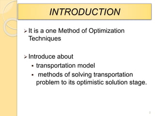
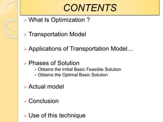
This presentation discusses transportation model optimization techniques. It introduces transportation models and methods for solving transportation problems to reach an optimal solution. Specifically, it covers what optimization is, transportation models and their applications, phases of solution such as obtaining initial and optimal solutions, and methods like the North-West Corner rule. It provides an example problem demonstrating solutions using different methods and showing the Vogel's Approximation Method achieves the lowest transportation cost. The presentation concludes that this technique can optimize scheduling, production, investment and other problems by minimizing transportation or distribution costs.

1. Presentation on
Transportation Model Methods of
Optimization Techniques
BY
SATISH AWARE (M.Tech Civil)

2. INTRODUCTION
It is a one Method of Optimization
Techniques
Introduce about
 transportation model
 methods of solving transportation
problem to its optimistic solution stage.
2

3.  What Is Optimization ?
 Transportation Model
 Applications of Transportation Model…
 Phases of Solution
Obtains the Initial Basic Feasible Solution
Obtains the Optimal Basic Solution
 Actual model
 Conclusion
 Use of this technique
CONTENTS

4. What Is Optimization ?
 Optimization problem :
Maximizing or minimizing some function
• Common
applications:
Minimal cost,
maximal profit,
minimal error,
optimal design,
optimal
management,
variation principles

5.  Transportation Model
 The transportation problem is a special type
of LPP
 The objective is to minimize the cost of
distributing a product
 Because of its special structure the usual
simplex method is not suitable
 require special method of solution.
 Aim : find out optimum transportation
schedule keeping in mind cost of
transportation to be minimized

6. Assumptions in the transportation
Model :
1. Total qty of the item available at different sources
is equal to the total requirement at different
destinations.
2. Item can be transported conveniently from all
sources to destinations.
3. The unit transportation cost of the item from all
sources to destinations is certainly & precisely
known.
4. The transportation cost on given route is directly
proportional to the no. of units shipped on that
route.
5. The objective is to minimize the total
transportation cost for the organization as a
whole & not for individual supply & distribution
centre.

7. Application of Transportation
Model
 Minimize shipping costs
 Determine low cost location
 Find minimum cost production
schedule
 Military distribution system

8.  Phases of Solution of Transportation
Problem :-
 Phase I- obtains the initial basic feasible
solution
◦ North West Corner Method (NWC)
◦ Row Minima Method
◦ Column Minima Method
◦ Least Cost Method
◦ Vogel's Approximation Method (VAM)
 Phase II-obtains the optimal basic solution
◦ Stepping Stone Method
◦ Modified Distribution Method a.k.a. MODI
Method

9. Example.
 Factory takes 16 Rs/km transport cost per truck
for supply of bricks.
 Following is requirement of bricks on various
sites with respective distances(km) from
warehouses
 Available Single truck contains 7000 bricksSites 
warehouse
s

Karad Saidapur Masur
Agashiv
Nagar
Available
Bricks
Tasavde 2 3 11 7 42,000
Tembhu 1 0 6 1 7,000
Koparde 5 8 15 9 70,000
Required
Bricks
49,000 35,000 21,000 14,000 1,19,000

10. Solution 
Unit cost of single tuck transport =17x travelling
distance(km)
Sites 
warehouses

Karad Saidapur Masur
Agashiv
Nagar
Available
Bricks
(trucks)
Tasavde 2 3 11 7 6
Tembhu 1 0 6 1 1
Koparde 5 8 15 9 10
Required
Bricks (trucks)
7 5 3 2 17*

11. 1) NWC:
2 3 11 7 6
1 0 6 1 1
5 8 15 9 10
7
1
5 3 2 17*
Transport distance =(2x6)+(1x1)+(8x5)+(15x3)+(9x2)=116 km
Transport Cost =116x16=1856 Rs.

12. 2) LCM :
Bricks
Factory
Karad Saidapur Masur
Agashiv
Nagar
Available Bricks
(trucks)
Tasavde 2 3 11 7 6
Tembhu 1 0 6 1 1
Koparde 5 8 15 9 10
Required
Bricks
(trucks)
7
1
5
4
3 2
17*
Transport distance =(0x1)+(2x6)+(5x1)+(8x4)+(15x3)+(9x2)=112
km
Transportation Cost = 112x16 = 1792 Rs.

13. 3) VAM :
Bricks
Factory
Karad Saidapur Masur
Agashiv
Nagar
Available
Bricks
(trucks)
penalties
Tasavde 2 3 11 7 6 1 1 5
Tembhu 1 0 6 1 1 . 1 .
Koparde 5 8 15 9 10 . 3 4
Required
Bricks
(trucks)
7
6
5 3 2
1
17*
penalties
1
3
3
5
5
4
6
2
Transport distance =(1x1)+(3x5)+(2x1)+(5x6)+(15x3)+(9x1)=102
km

14.  IBFS by VAM & check
optimality:
2 3 11 7
1 5
1 0 6 1
1
5 8 15 9
6 3 1
 Modified Distribution
Method :-
2
-3
5
0 1 10 4
A
B
C
P Q R S
Cell Values =Cell Amount –U-V
AR= 11-2-10= -1
AS= 7-2-4 =1
BP= 1-(-3)-0 =4
BQ= 0- (-3)-1 =2
BR= 6- (-3)-10 = -1
CQ= 8-5-1 =2
1ST TRIAL :-
Allocated cells =Nc+Nr-1
Here 4+3-1=6_____we can check optimali

15. 1
-3
5
0 1 10 4
A
B
C
P Q R S
Cell Values =Cell Amount –U-V
AP= 2-1-0= 1
AS= 7-1-4 =2
BP= 1-(-3)-0 =4
BQ= 0- (-3)-1 =2
BR= 6- (-3)-10 = -1
CQ= 8-5-1 =2
2nd TRIAL :-
2 3 11 7
5 1
1 0 6 1
1
5 8 15 9
7 2 1

16. 2 3 11 7
5 1
1 0 6 1
1
5 8 15 9
7 1 2
Cell Values =Cell Amount –U-V
AP= 2-1-0= 1
AS= 7-1-4 =2
BP= 1-(-4)-0 =5
BQ= 0- (-4)-2 =2
BS= 1- (-4)-4 = 0
CQ= 8-5-2 =1
(NO ANY –ve CELL VALUE , IT IS OPTIMAL STAGE OF MODEL)
3nd TRIAL :-
1
-4
5
0 2 10 4
A
B
C
P Q R S
TRANSPORTATION DISTANCE =(3x5)+(11x1)+(6x1)+(5x7)+(15x1)+(9x2) = 100
km
TRANSPORTATION COST =100 x16=1600 Rs.

17. Conclusion :
NCM LCM VAM MODI
1856
1792
1632
1600
TOTAL COST(Rs.)

18.  Use of This Technique :-
This model can be used for a wide variety
of situations such as
scheduling, production, investment, mix
problems & many other, so that the model
is really not confined to transportation or
distribution only.
The objective is to minimize the cost of
transportation while meeting the
requirements at the destinations.