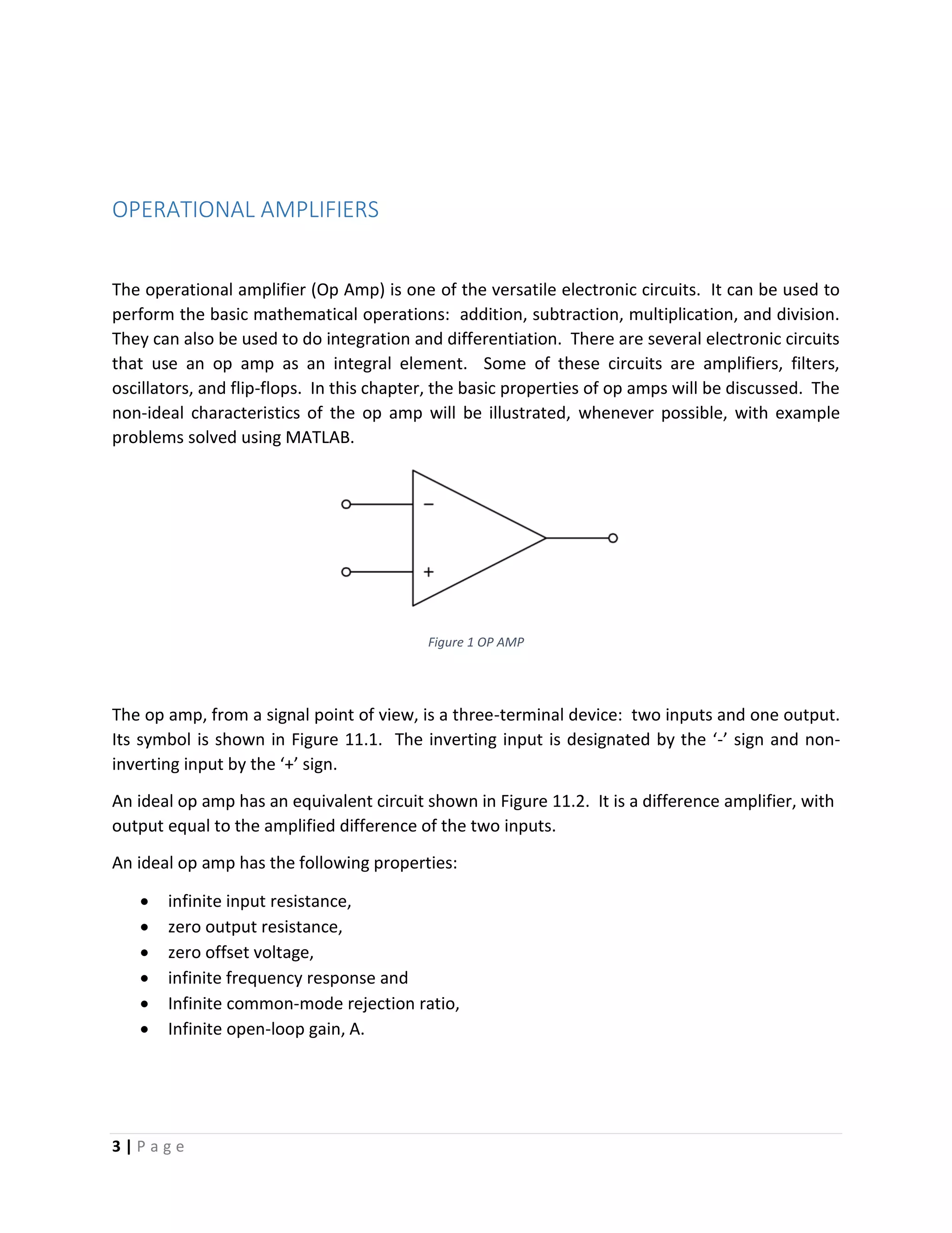
The document is a comprehensive project report on operational amplifiers (op amps), detailing their configurations, characteristics, modes, applications, and the use of MATLAB for simulating op amp circuits. It covers both inverting and non-inverting configurations, control functions, and practical applications such as PID controllers. Additionally, the report includes a bibliography and analysis of op amp circuits with MATLAB commands to demonstrate their functionality.

1. PROJECT REPORT
Operational amplifier (op amp) and its Requirements, Applications,
Modes, Circuit. Simulating and analyzing some op amp circuits on
MATLAB.
VI.6.2 Control Systems
Presented By: Harikesh
[140016]

2. 1 | P a g e
Acknowledgement
We have taken efforts in this project. However, it would not have been possible without the kind
support and help of many individuals. We would like to extend our sincere thanks to all of them. We are
highly indebted Dr. HARENDRA PAL for his guidance and constant supervision as well as for providing
necessary information regarding the project& also for their support in completing the project.

3. 2 | P a g e
Contents
Acknowledgement........................................................................................................................................1
OPERATIONAL AMPLIFIERS...........................................................................................................................3
INVERTING CONFIGURATION........................................................................................................................5
NON-INVERTING CONFIGURATION...............................................................................................................7
Typical Op Amp Control Functions ...............................................................................................................9
Gain...........................................................................................................................................................9
Integration ..............................................................................................................................................10
Differentiation.........................................................................................................................................10
Proportional-Integral-Derivative Controller ...........................................................................................11
Transfer function from the Op-amp circuit: ...............................................................................................12
SIMULINK ....................................................................................................................................................14
Non-Inverting Amplifier Using Operational Amplifier ............................................................................14
Adder Using OP- Amp .............................................................................................................................15
Inverting Op-Amp Circuit........................................................................................................................16
Finite Gain Op-Amp.................................................................................................................................16
Analysis of Op Amp Circuits Using MATLAB................................................................................................17
MATLAB Commands ...............................................................................................................................18
FINDING Poles and Zeroes and Plotting Frequency Response ...............................................................19
MATLAB Code .....................................................................................................................................20
CONCLUSION...............................................................................................................................................21
Bibliography ................................................................................................................................................22

4. 3 | P a g e
OPERATIONAL AMPLIFIERS
The operational amplifier (Op Amp) is one of the versatile electronic circuits. It can be used to
perform the basic mathematical operations: addition, subtraction, multiplication, and division.
They can also be used to do integration and differentiation. There are several electronic circuits
that use an op amp as an integral element. Some of these circuits are amplifiers, filters,
oscillators, and flip-flops. In this chapter, the basic properties of op amps will be discussed. The
non-ideal characteristics of the op amp will be illustrated, whenever possible, with example
problems solved using MATLAB.
Figure 1 OP AMP
The op amp, from a signal point of view, is a three-terminal device: two inputs and one output.
Its symbol is shown in Figure 11.1. The inverting input is designated by the ‘-’ sign and non-
inverting input by the ‘+’ sign.
An ideal op amp has an equivalent circuit shown in Figure 11.2. It is a difference amplifier, with
output equal to the amplified difference of the two inputs.
An ideal op amp has the following properties:
 infinite input resistance,
 zero output resistance,
 zero offset voltage,
 infinite frequency response and
 Infinite common-mode rejection ratio,
 Infinite open-loop gain, A.

5. 4 | P a g e
Figure 2Equivalent Circuit of an Ideal Op Amp
A practical op amp will have large but finite open-loop gain in the range from 105 to 109. It also
has a very large input resistance 106 to 1010 ohms. The output resistance might be in the range
of 50 to 125 ohms. The offset voltage is small but finite and the frequency response will deviate
considerably from the infinite frequency response. The common-mode rejection ratio is not
infinite but finite.
Figure 3 Negative Feedback Connections for Op Amp (a) Inverting (b) Non-inverting configuration

6. 5 | P a g e
With negative feedback and finite output voltage, Figure 2 shows that
Vo = A(V2 – V1) (1.1)
Since the open-loop gain is very large,
(V2-V1) =
𝑉𝑜
𝐴
≈ 0 (1.2)
Equation (1.2) implies that the two input voltages are also equal. This condition is termed the
concept of the virtual short circuit. In addition, because of the large input resistance of the op
amp, the latter is assumed to take no current for most calculations.
INVERTING CONFIGURATION
An op amp circuit connected in an inverted closed loop configuration is shown in Figure 4
Figure 4 Inverting Configuration of an Op Amp
Using nodal analysis at node A, we have
𝑉𝑎−𝑉𝑖𝑛
𝑍1
+
𝑉𝑎−𝑉𝑜
𝑍2
+ 𝐼1 = 0 (1.3)
From the concept of a virtual short circuit,
Va = Vb = 0 (1.4)
And because of the large input resistance, I1 = 0. Thus, Equation (11.3) simplifies to
𝑉𝑜
𝑉𝑖𝑛
= −
𝑍2
𝑍1
(1.5)

7. 6 | P a g e
The minus sign implies that VIN and V0 are out of phase by 180o. The input impedance, ZIN, is
given as
ZIN =
𝑉𝐼𝑁
𝐼1
= 𝑍1 (1.6)
If Z1 = R1 and Z2 = R2 , we have an inverting amplifier shown in Figure 5.
Figure 5 Inverting amplifier
The closed-loop gain of the amplifier is
𝑉𝑜𝑛
𝑉𝑖𝑛
= −
𝑅2
𝑅1
(1.7)
And the input resistance is R1. Normally, R2 > R1 such that |Vo|> |VIN|.
With the assumptions of very large open-loop gain and high input resistance, the closed-loop
gain of the inverting amplifier depends on the external components R1, R2, and is independent
of the open-loop gain.
For Figure 4, if Z1 = R1 and Z2 =
1
𝑗𝑤𝑐
,
We obtain an integrator circuit shown in Figure 6. The closed-loop gain of the integrator is
𝑉𝑜
𝑉𝑖𝑛
=
1
𝑗𝑤𝐶𝑅1
(1.8)
Figure 6 Op Amp Inverting Integrator

8. 7 | P a g e
NON-INVERTING CONFIGURATION
An op amp connected in a non-inverting configuration is shown in Figure 7.
Figure 7 Non-Inverting Configuration
Using nodal analysis at node A
𝑉𝑎
𝑍1
+
𝑉𝑎−𝑉𝑜
𝑍2
+ 𝐼1 = 0 (1.9)
From the concept of a virtual short circuit,
VIN = Va (1.10)
And because of the large input resistance (i1 = 0 ), Equation (1.9) simplifies to
𝑉𝑜
𝑉𝑖𝑛
= 1 +
𝑍2
𝑍1
(1.11)
The gain of the inverting amplifier is positive. The input impedance of the amplifier ZIN
approaches infinity, since the current that flows into the positive input of the op-amp is almost
zero.
If Z1 = R1 and Z2 = R2, becomes a voltage follower with gain. This is shown in Figure 10.
Figure 8 Voltage Follower with Gain

9. 8 | P a g e
The Voltage gain is
𝑉𝑜
𝑉𝑖𝑛
= 1 +
𝑅2
𝑅1
(1.12)

10. 9 | P a g e
Typical Op Amp Control Functions
 Gain
 Integration
 Differentiation
 PI Controller
 PD Controller
 PID Controller
Gain
Figure 9 Gain Amplifier
 Used in closed loop control systems.
 Represents the relationship between the input and output signals commonly expressed
amplitude of the output divided by the input signals.
 Op amp most commonly represented as either an Inverting or Non-inverting amplifier.
 Inverting amplifiers change the sign and the level of the input signal.
 Non-inverting amplifier circuit can increase the size of the signal, remain the same, but it cannot
decrease.

11. 10 | P a g e
Integration
Figure 10 Integration Amplifier
 Utilized in controls to eliminate steady state error in closed loop systems.
 The integral mode changes the output of a control signal by an amount proportional to the
integral of the error.
 The Integrating op amp produces an output that is proportional to the integral of the input
voltage.
Differentiation
Figure 11 Differentiation Amplifier

12. 11 | P a g e
 The derivative control changes the output of a control signal proportionally to the rate of
change of the error signal.
 Method of error control is needed to help anticipate variations in the measure variable, set
point, or both by means of observing the rate of change of the error.
 The differentiator op amp produces an output that is proportional to the rate of change of the
input voltage.
Proportional-Integral-Derivative Controller
Figure 12 PD Amplifier
 The PID control is a combination of the proportional, integral, and derivative controls modes.
 Used on processes with sudden, large load changes when one or two control mode control is not
capable of keeping error within acceptable ranges.
 Integral mode eliminates the proportional offset caused by large load changes.
 Derivative mode reduces the tendency toward oscillations and provides a control action that
anticipates changes in the error signal.
 The PID op amp produces an output that is an accumulation of the error from the proportional,
integral, and derivative modes.

13. 12 | P a g e
Transfer function from the Op-amp circuit:
If we consider an ideal Op Amp, there is no current flow in the inverting input (see Figure 2).
Therefore, I0 = 0A and I2 and I1 are equal.
I2= I1
Moreover, being an ideal Op Amp, its gain is high, so the inverting input is at a virtual ground.
Figure 13 Ideal Op amp
Using the previous equation, we can replace I1 and I2 as follows:
Rearranging this equation and considering V = 0V, the transfer function of the inverting amplifier is
Transfer Function for the below Op amp circuit having R1 = 1000Ω, R3 =10000Ω, R4 =100000 Ω
And C3 = 1.0E-9F, C4 = 1.0E-7F

14. 13 | P a g e
𝐺(𝑠) =
s2
+ 1111000𝑠 + 1010000000
s2 + 111000𝑠 + 10000000

15. 14 | P a g e
SIMULINK
Non-Inverting Amplifier Using Operational Amplifier

16. 15 | P a g e
Adder Using OP- Amp

17. 16 | P a g e
Inverting Op-Amp Circuit
Finite Gain Op-Amp

18. 17 | P a g e
Analysis of Op Amp Circuits Using MATLAB
Model the operational amplifier as an ideal op amp. Then the output voltage of the inverting amplifier is
related to the input voltage by
Vo t = -
𝑅2
𝑅1
𝑉𝑠(𝑡)
Suppose that R1 = 2 kOhms , R2 = 50 kOhms , and vs = approx. 4 cos (2000p t) V. Using these values in
above Eq. Gives Vo(t) = 100 cos (2000p t) V. This is not a practical answer, it is likely that the operational
amplifier saturates, and, therefore, the ideal op amp is not an appropriate model of the operational
amplifier. When voltage saturation is included in the model of the operational amplifier, the inverting
amplifier is described by
Where Vs(t) denotes the saturation voltage of the operational amplifier.
Figures Below illustrate the use of MATLAB to analyze the inverting amplifier when the operational
amplifier model includes voltage saturation. Figure Below shows the resulting plot of the input and
output voltages of the inverting amplifier.

19. 18 | P a g e
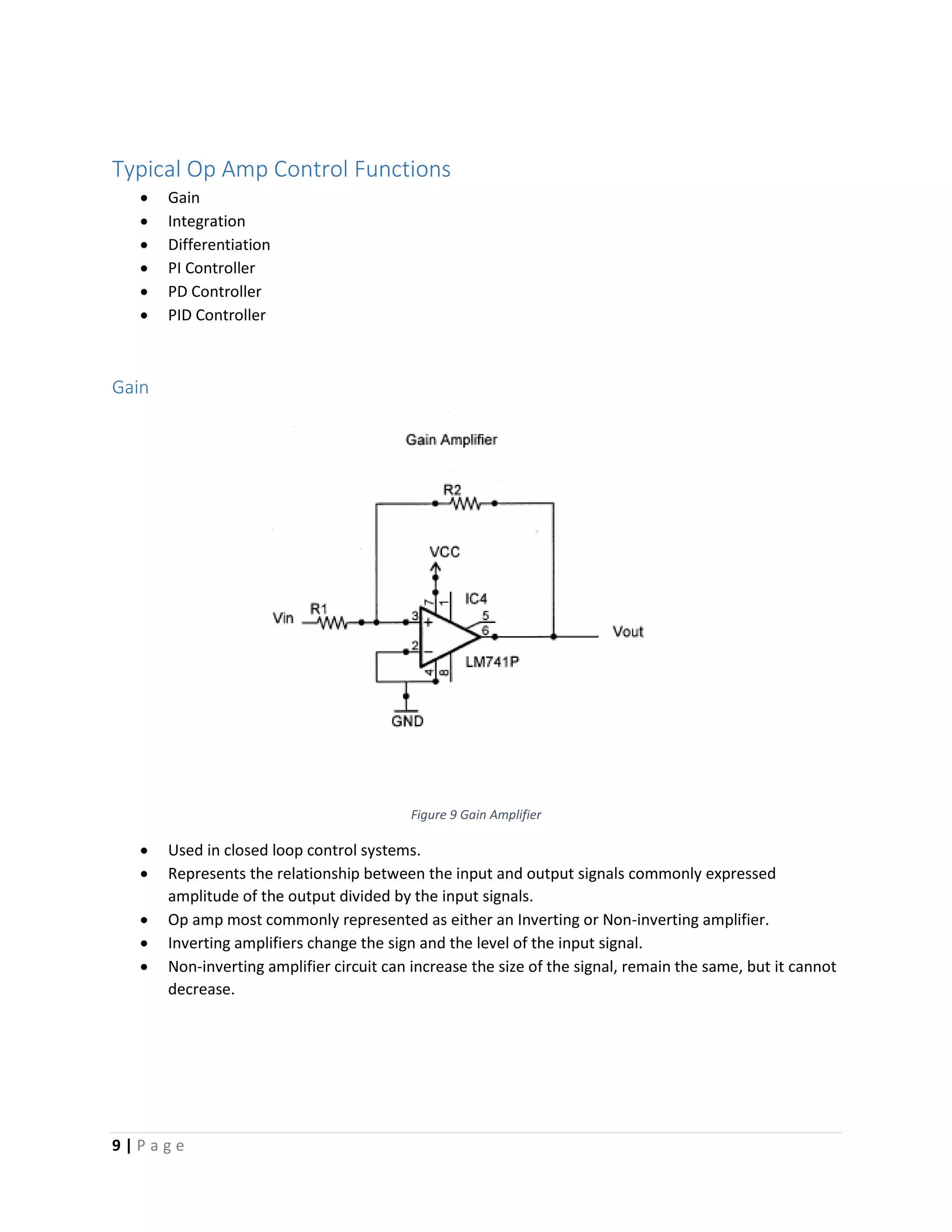
MATLAB Commands
>> R1 = 2e3; R2 = 50e3; R3 = 20e3;
>> vsat = 15;
>> M = 4; f = 1000; w = 2*pi*f;
>> theta = (pi/180) * 180;
>> tf = 2/f
tf =
0.0020
>> N = 200
N =
200
>> t = 0:tf/N:tf;
>> t = linspace(0, 2/f, 201);
>> vs = M*cos(w*t+theta);
>> for k=1:length(vs)
if (-(R2/R1)*vs(k) < -vsat)
vo(k) = -vsat;
else if (-(R2/R1)*vs(k) > vsat)
vo(k) = vsat;
else
vo(k) = -(R2/R1) * vs(k);
end
end
end
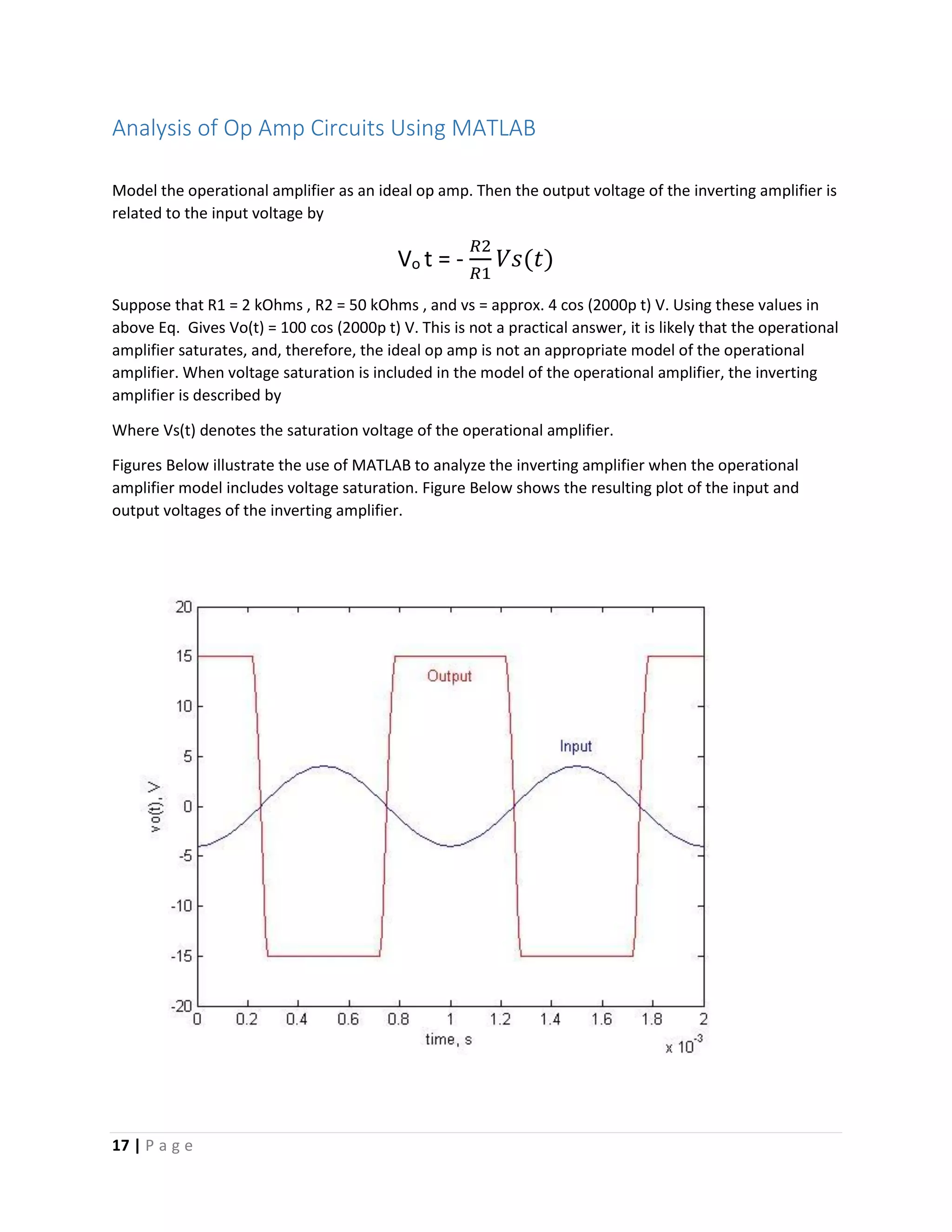
>> plot(t, vo, 'r', t, vs, 'b')
>> axis([0 tf -20 20])
>> xlabel('time, s')
>> ylabel('vo(t), V')
>> text(1e-3,13,'Output', ...
'HorizontalAlignment',...
'center', 'Color', [1 0 0]);
>> text(1.5e-3,6,'Input', ...
'HorizontalAlignment',...
'center', 'Color', [0 0 1]);

20. 19 | P a g e
FINDING Poles and Zeroes and Plotting Frequency Response

21. 20 | P a g e
MATLAB Code
% Poles and zeros, frequency response
c1 = 1e-7;
c2 = 1e-3;
r1 = 10e3;
r2 = 10;
% poles and zeros
b1 = c2*r2;
a1 = c1*r1;
num = [b1 1];
den = [a1 1];
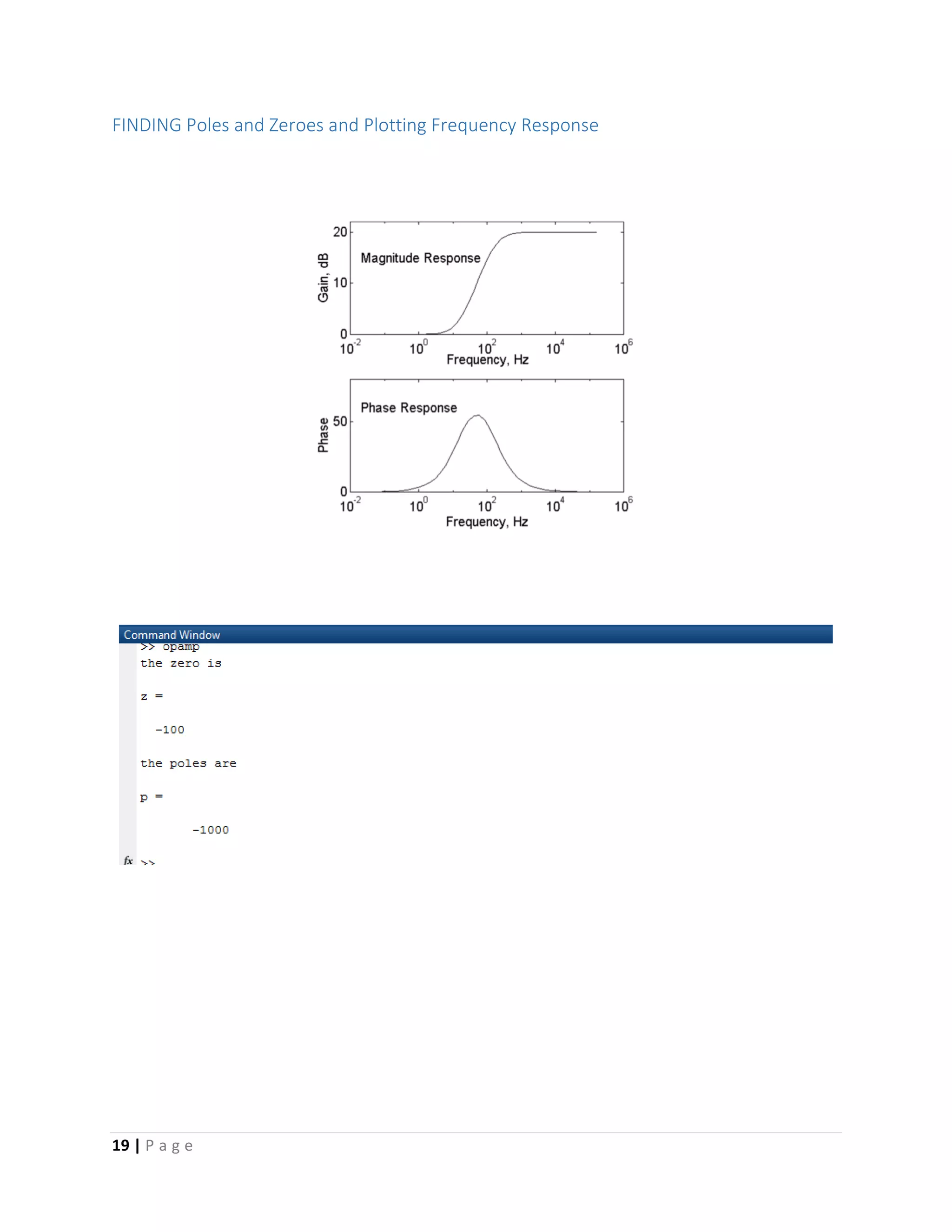
disp('the zero is')
z = roots(num)
disp('the poles are')
p = roots(den)
% the frequency response
w = logspace(-2,6);
h = freqs(num,den,w);
gain = 20*log10(abs(h));
f = w/(2*pi);
phase = angle(h)*180/pi;
subplot(211),semilogx(f,gain,'w');
xlabel('Frequency, Hz')
ylabel('Gain, dB')
axis([1.0e-2,1.0e6,0,22])
text(2.0e-2,15,'Magnitude Response')
subplot(212),semilogx(f,phase,'w')
xlabel('Frequency, Hz')
ylabel('Phase')
axis([1.0e-2,1.0e6,0,75])
text(2.0e-2,60,'Phase Response')

22. 21 | P a g e
CONCLUSION
Op-amps are extremely important electronic devices that facilitate the use of output signals. By using a
ratio of two resistors to achieve a desired gain, an output Voltage proportionate to the input Voltage
can be determined and measured. The tests done for this experiment show the accuracy and preferred
output that can be attained through the use of an op-amp.

23. 22 | P a g e
Bibliography
 Histand, Michael B., and Alciatore, David G., Introduction to Mechatronics and Measurement
Systems, WCB/McGraw-Hill, Boston, MA, 1999.
 Soper, Jon A., “Electrical Engineering Basics” in Principles and Practice of Electrical Engineering,
Merle C. Potter, ed., Great Lakes Press, Inc., Ann Arbor, Michigan, 1998.
 Rizzoni, Giorgio, Principles and Applications of Electrical Engineering, 3rd
edition, McGraw-Hill,
Boston, MA, 2000.
 Norman.Nise - Control.Systems.Engineering.6th.Edition
 Mathworks { https://in.mathworks.com}