Download to read offline


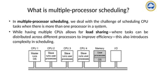
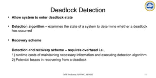
![Dr.M.Sivakumar, AP/NWC, SRMIST 21
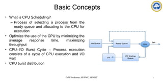
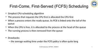
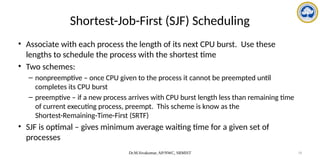
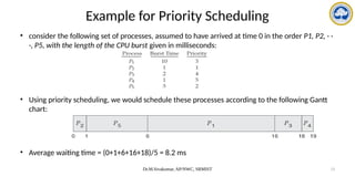
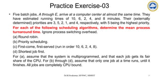
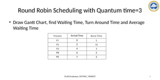
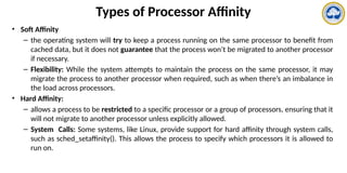
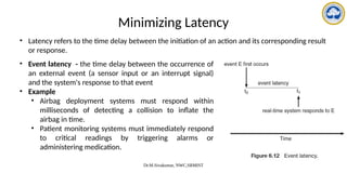
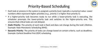
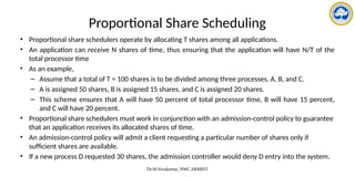
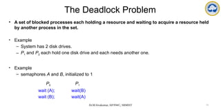
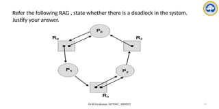
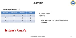
Example Preemptive SJF
• consider the following four processes, with the length of the CPU burst given in milliseconds:
• preemptive SJF schedule is as depicted in the following Gantt chart:
• The average waiting time = [(10-1-0) + (1-1) + (17-2) + (5-3)] / 4
= (9+0+15+2)/4 = 26/4 = 6.5 ms](https://image.slidesharecdn.com/operatingsystemscpuscheduling-241118113036-3be17652/85/Operating-Systems-CPU-Scheduling-and-its-Algorithms-21-320.jpg)

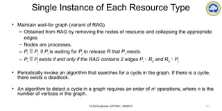
![Dr.M.Sivakumar, AP/NWC, SRMIST 26
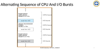
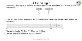
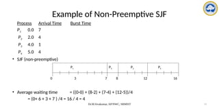
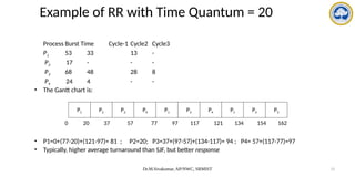
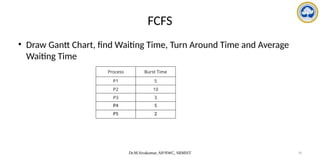
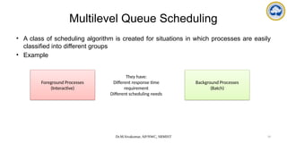
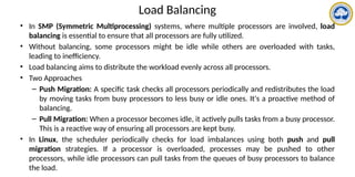
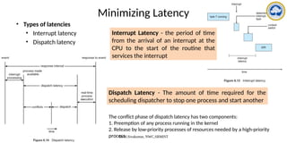
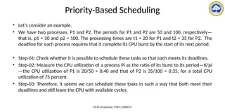
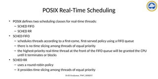
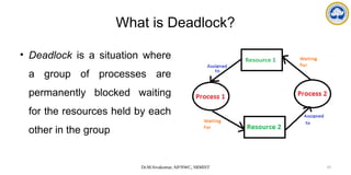
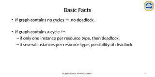
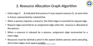
Example of RR with Time Quantum = 4
• Consider the following set of processes that arrive at time 0, with the length of the CPU burst
given in milliseconds:
• The resulting RR schedule is as follows:
• The average waiting time = [(10-4) + 4 + 7] / 4 = 17/4 = 5.66 ms](https://image.slidesharecdn.com/operatingsystemscpuscheduling-241118113036-3be17652/85/Operating-Systems-CPU-Scheduling-and-its-Algorithms-26-320.jpg)
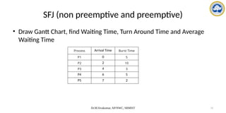
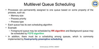


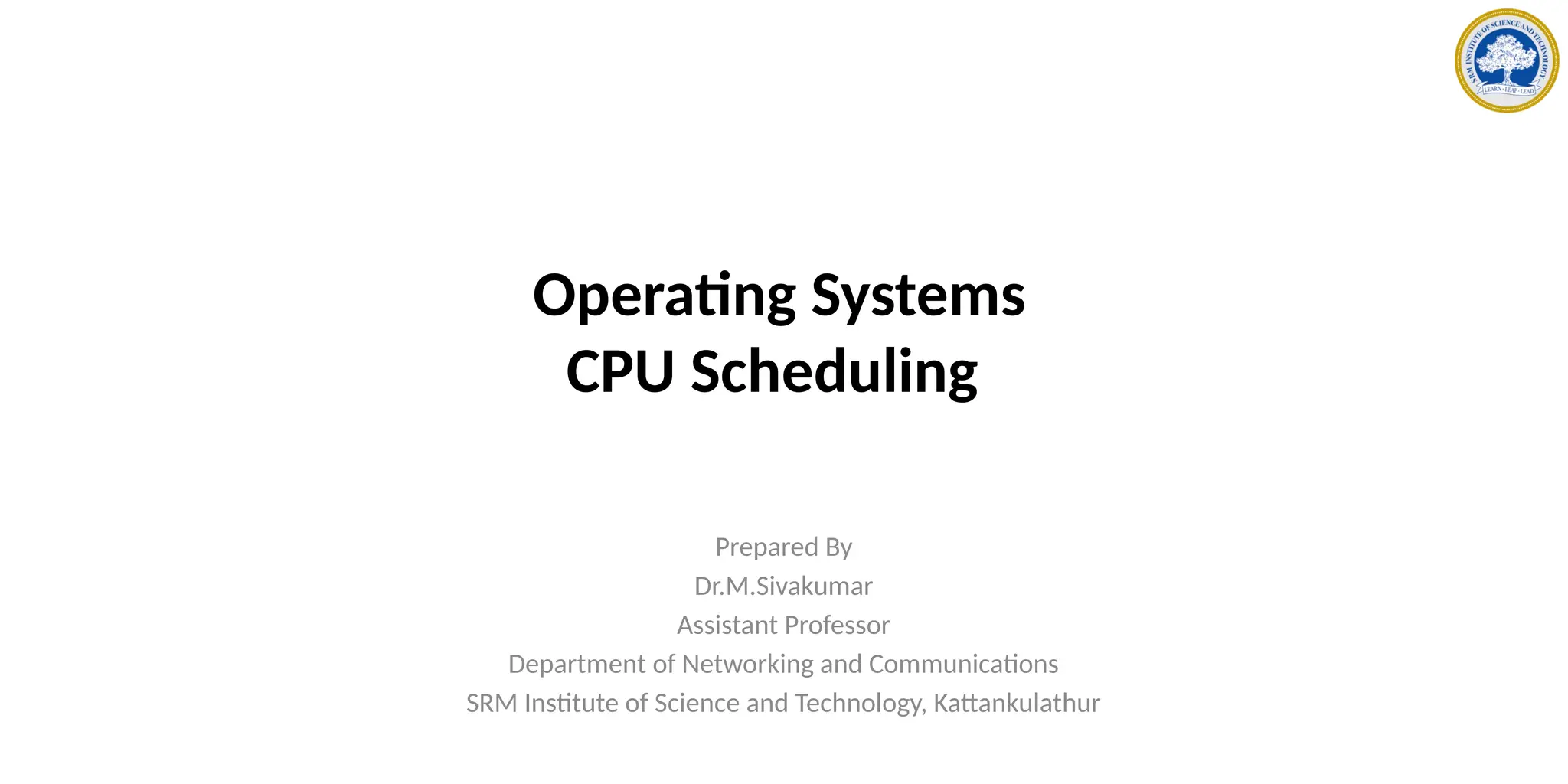
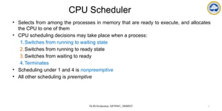
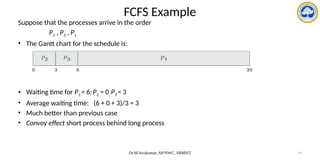
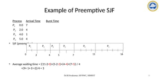
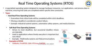
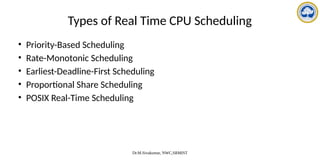
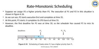
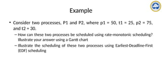
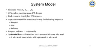
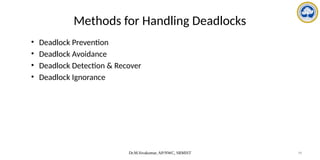
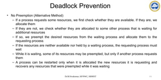
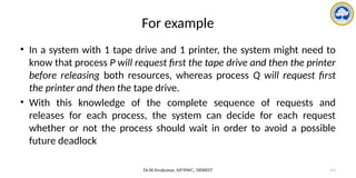
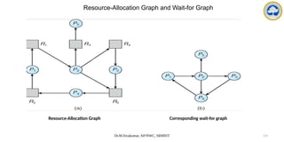
![Pthread scheduling API
#include <pthread.h>
#include <stdio.h>
#define NUM THREADS 5
int main(int argc, char *argv[])
{
int i, scope;
pthread t tid[NUM THREADS];
pthread attr t attr;
/* get the default attributes */
pthread attr init(&attr);
/* first inquire on the current scope */
if (pthread attr getscope(&attr, &scope) != 0)
fprintf(stderr, "Unable to get scheduling scopen");
else {
if (scope == PTHREAD SCOPE PROCESS)
printf("PTHREAD SCOPE PROCESS");
else if (scope == PTHREAD SCOPE SYSTEM)
printf("PTHREAD SCOPE SYSTEM");
else
fprintf(stderr, "Illegal scope value.n");
}
/* set the scheduling algorithm to PCS or SCS */
pthread attr setscope(&attr, PTHREAD SCOPE SYSTEM);
/* create the threads */
for (i = 0; i < NUM THREADS; i++)
pthread create(&tid[i],&attr,runner,NULL);
/* now join on each thread */
for (i = 0; i < NUM THREADS; i++)
pthread join(tid[i], NULL);
}
/* Each thread will begin control in this function */
void *runner(void *param)
{
/* do some work ... */
pthread exit(0);
}](https://image.slidesharecdn.com/operatingsystemscpuscheduling-241118113036-3be17652/85/Operating-Systems-CPU-Scheduling-and-its-Algorithms-46-320.jpg)


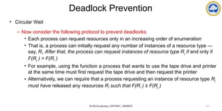

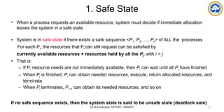


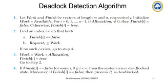
![Dr.M.Sivakumar, AP/NWC, SRMIST 122
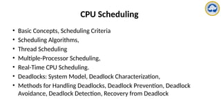
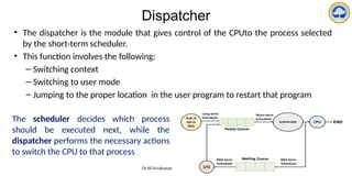
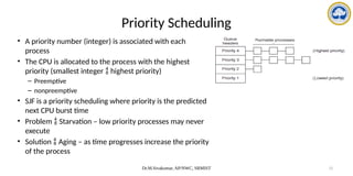
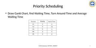
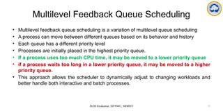
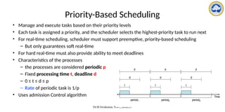
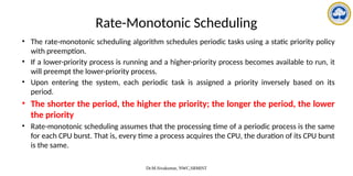
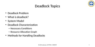
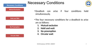
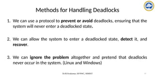
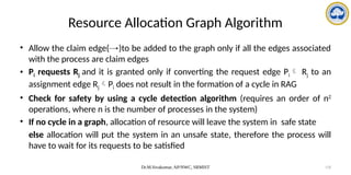
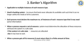
Data Structures for the Banker’s Algorithm
• Available: Vector of length m. If available [j] = k, there are k instances of resource type
Rj available.
• Max: n x m matrix. If Max [i,j] = k, then process Pi may request at most k instances of
resource type Rj.
• Allocation: n x m matrix. If Allocation[i,j] = k then Pi is currently allocated k instances
of Rj.
• Need: n x m matrix. If Need[i,j] = k, then Pi may need k more instances of Rj to
complete its task.
Need [i,j] = Max[i,j] – Allocation [i,j].
To encode the state of Resource Allocation
Let n = number of processes, and m = number of resources types.](https://image.slidesharecdn.com/operatingsystemscpuscheduling-241118113036-3be17652/85/Operating-Systems-CPU-Scheduling-and-its-Algorithms-122-320.jpg)
![Dr.M.Sivakumar, AP/NWC, SRMIST 123
• Data structures – vary over time in both size and value
• To simplify the process of banker’s alg.
X,Y vectors of length n
X<=Y only if X[i] <= Y[i] for all i=1,2…n
• Treat each row in the matrices Allocation and Need as vectors namely,
Allocationi – resources currently allocated to Pi
Needi – additional resource that Pi may still request to complete its task](https://image.slidesharecdn.com/operatingsystemscpuscheduling-241118113036-3be17652/85/Operating-Systems-CPU-Scheduling-and-its-Algorithms-123-320.jpg)
![Dr.M.Sivakumar, AP/NWC, SRMIST 124
Safety Algorithm
1. Let Work and Finish be vectors of length m and n, respectively.
Initialize: Work = Available and Finish [i] = false for i = 0, 1, …, n- 1.
2. Find an index i such that both:
(a) Finish [i] == false
(b) Needi Work
If no such i exists, go to step 4.
3. Work = Work + Allocationi
Finish[i] = true
go to step 2.
4. If Finish [i] == true for all i, then the system is in a safe state.
Safety algorithm may require an order of mxn2
operations to decide whether a state is safe](https://image.slidesharecdn.com/operatingsystemscpuscheduling-241118113036-3be17652/85/Operating-Systems-CPU-Scheduling-and-its-Algorithms-124-320.jpg)
![Dr.M.Sivakumar, AP/NWC, SRMIST 125
Resource-Request Algorithm for Process Pi
Requesti = request vector for process Pi.
If Requesti [j] = k then process Pi wants k instances of resource type Rj.
• If safe the resources are allocated to Pi.
• If unsafe Pi must wait, and the old resource-allocation state is restored](https://image.slidesharecdn.com/operatingsystemscpuscheduling-241118113036-3be17652/85/Operating-Systems-CPU-Scheduling-and-its-Algorithms-125-320.jpg)
![Dr.M.Sivakumar, AP/NWC, SRMIST 134
Several Instances of a Resource Type
• Available: A vector of length m indicates the number of available resources of each
type.
• Allocation: An n x m matrix defines the number of resources of each type currently
allocated to each process.
• Request: An n x m matrix indicates the current request of each process. If Request
[ij] = k, then process Pi is requesting k more instances of resource type. Rj.](https://image.slidesharecdn.com/operatingsystemscpuscheduling-241118113036-3be17652/85/Operating-Systems-CPU-Scheduling-and-its-Algorithms-134-320.jpg)
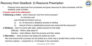
![Dr.M.Sivakumar, AP/NWC, SRMIST 136
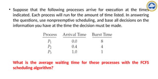
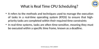
Example of Detection Algorithm
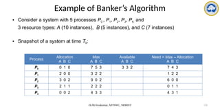
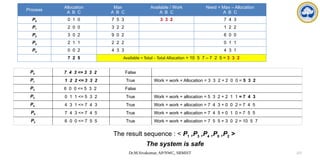
• Five processes P0 through P4;three resource types
A = 7 instances, B = 2 instances, and C =6 instances
• Snapshot at time T0:
Allocation Request Available
A B C A B C A B C
P0 0 1 0 0 0 0 0 0 0
P1 2 0 0 2 0 2
P2 3 0 3 0 0 0
P3 2 1 1 1 0 0
P4 0 0 2 0 0 2
• Sequence <P0, P2, P3, P1, P4> will result in Finish[i] = true for all i.](https://image.slidesharecdn.com/operatingsystemscpuscheduling-241118113036-3be17652/85/Operating-Systems-CPU-Scheduling-and-its-Algorithms-136-320.jpg)
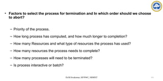

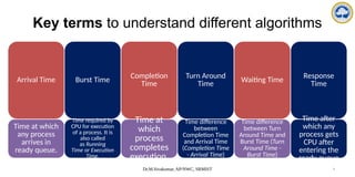
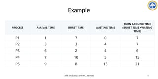
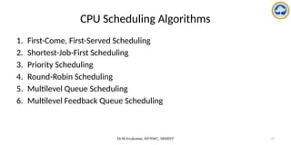
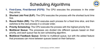
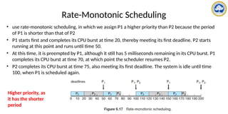
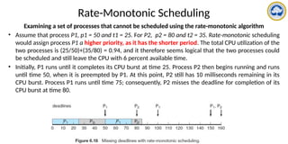
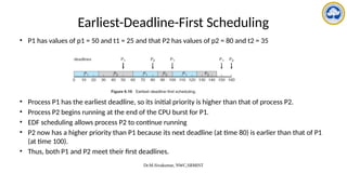
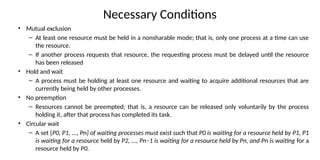
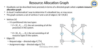
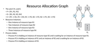
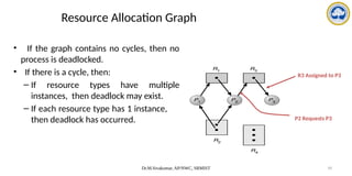
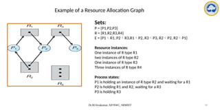
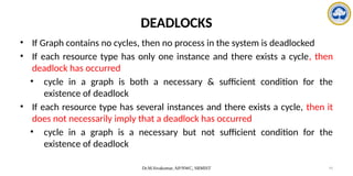
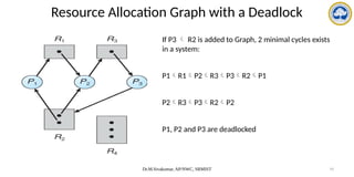
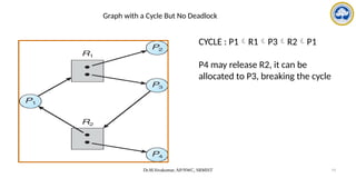
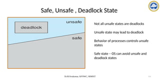
The document discusses CPU scheduling, covering essential concepts, criteria, algorithms, and the management of deadlocks. It details various scheduling algorithms such as First-Come-First-Served, Shortest Job First, Priority Scheduling, and Round Robin, each with explanations of their mechanics and examples. Additionally, the document addresses issues like preemptive vs non-preemptive scheduling and introduces advanced concepts like multilevel queue and multilevel feedback queue scheduling.