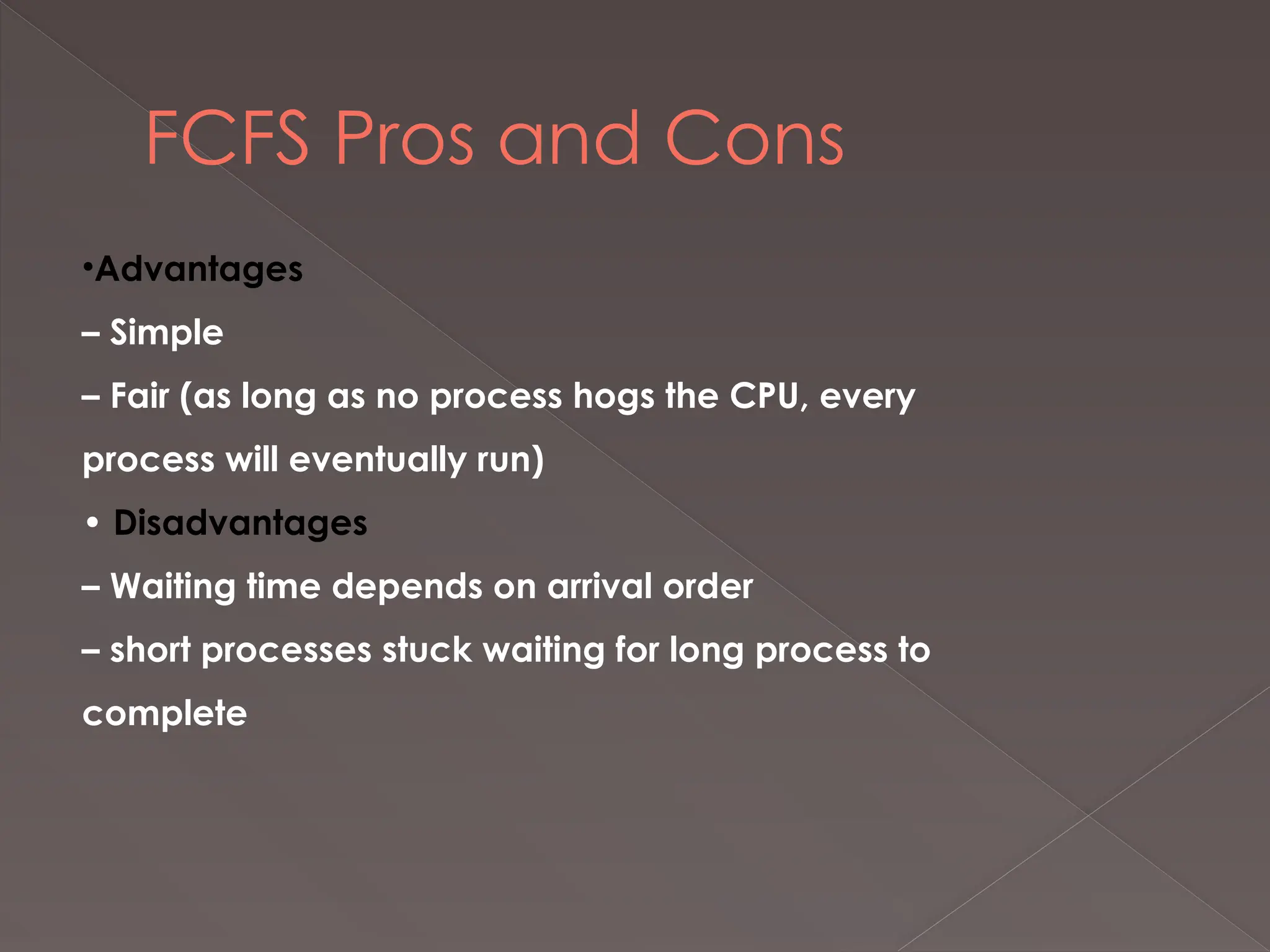
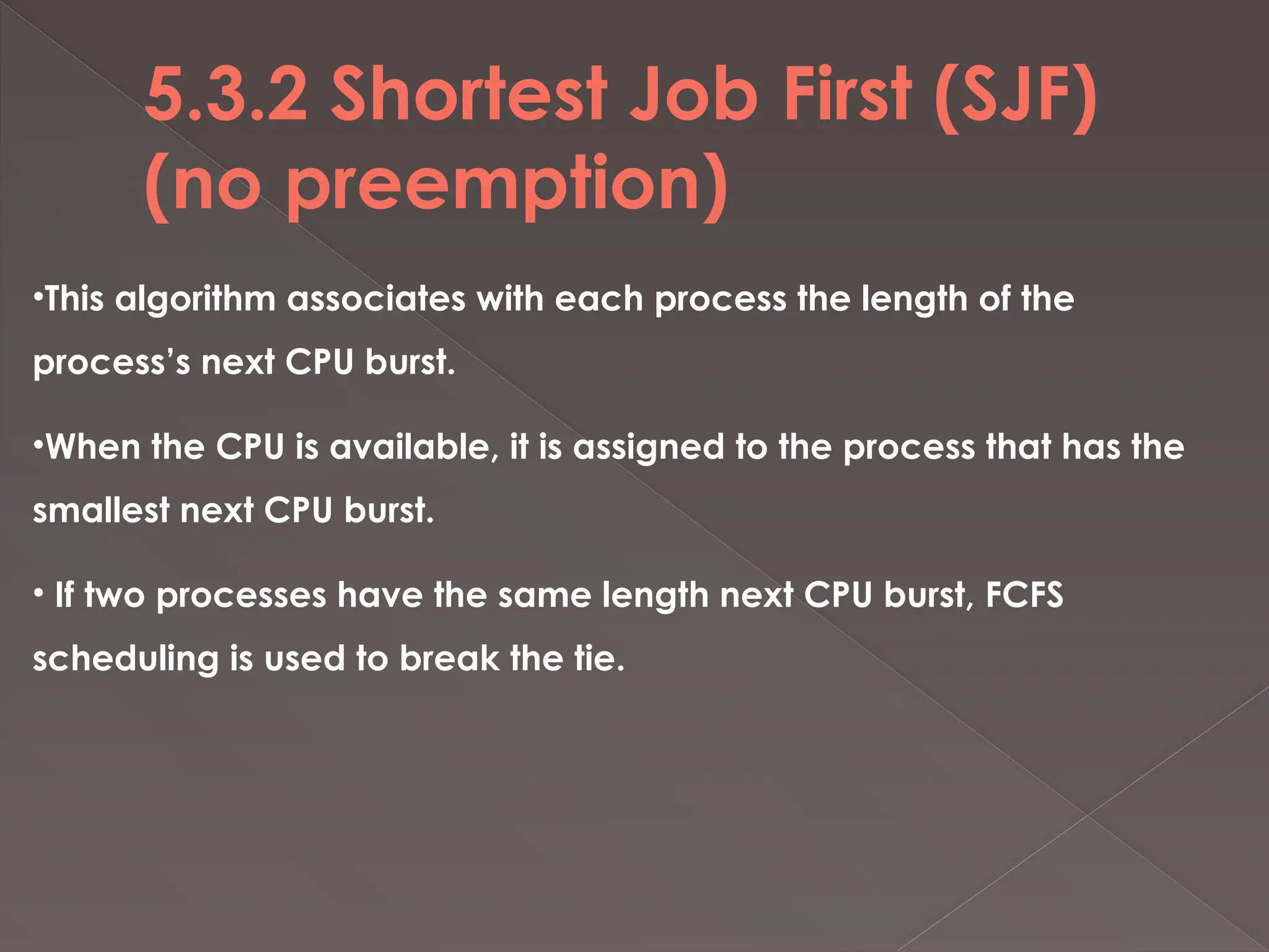
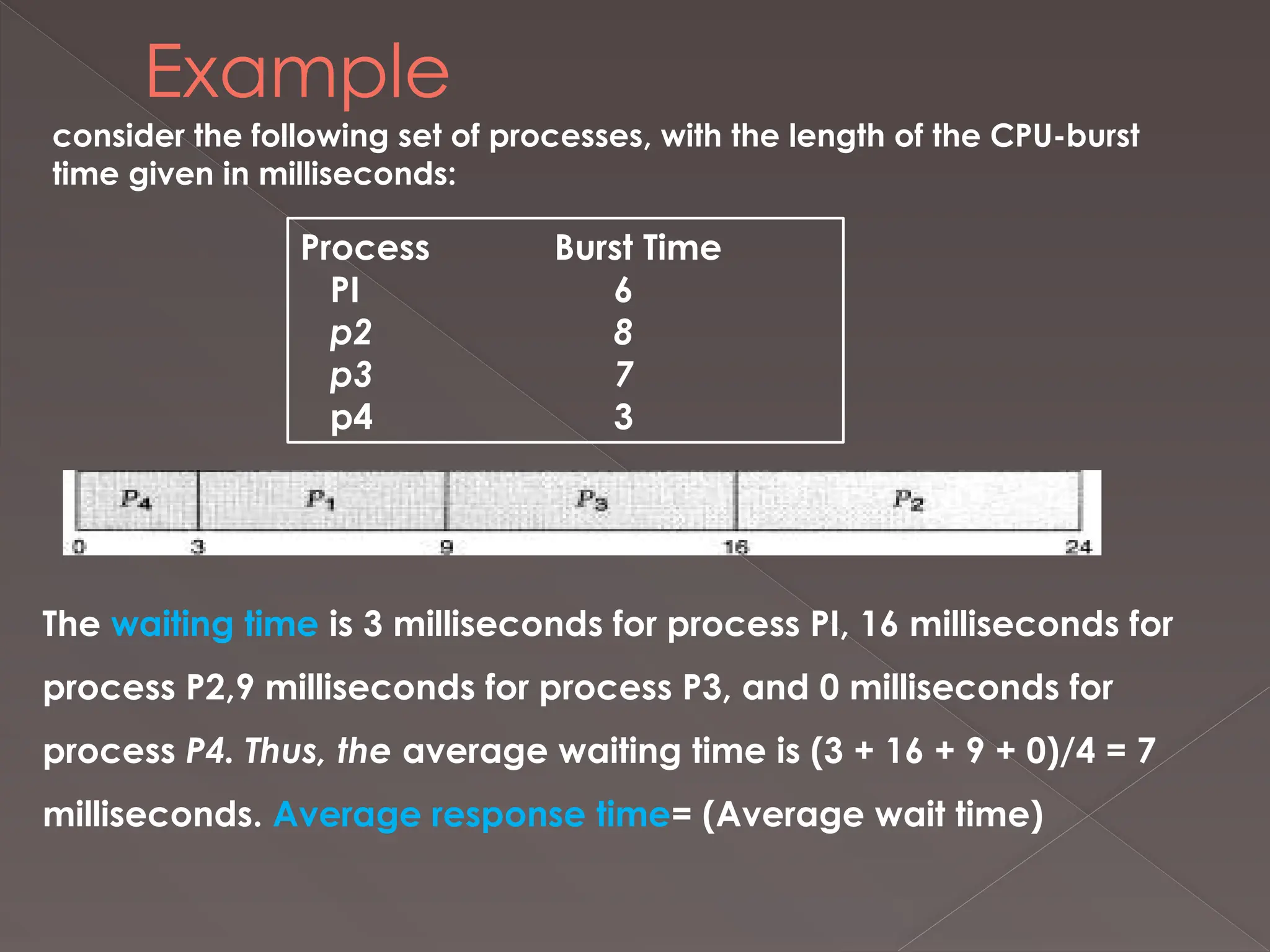
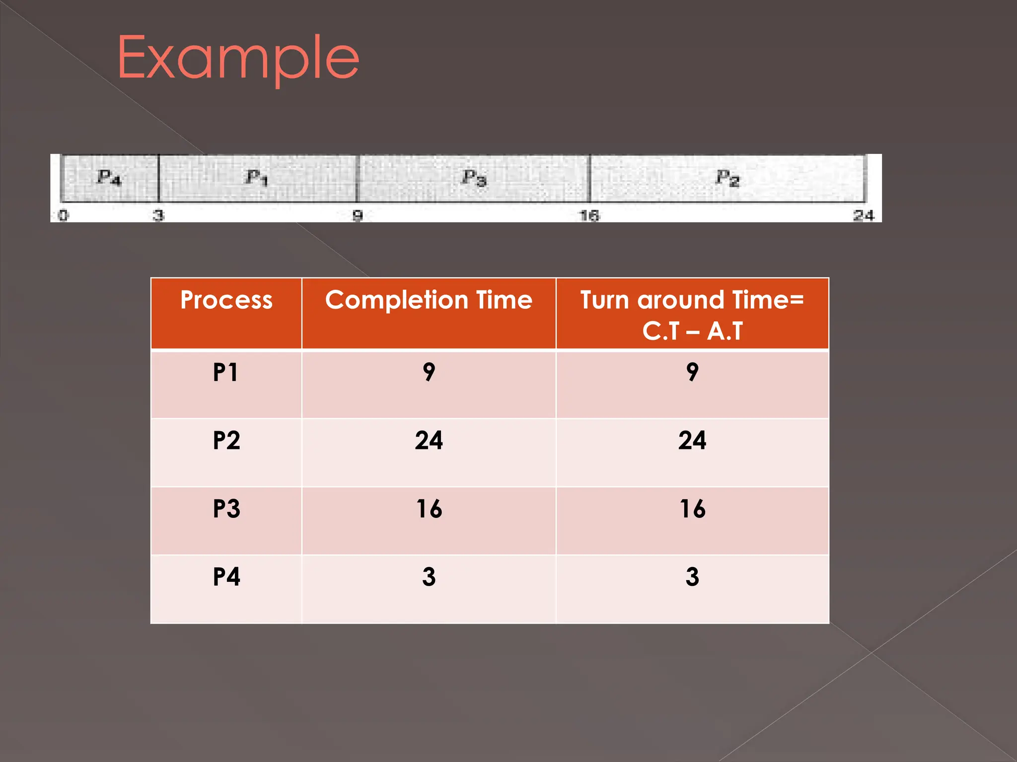
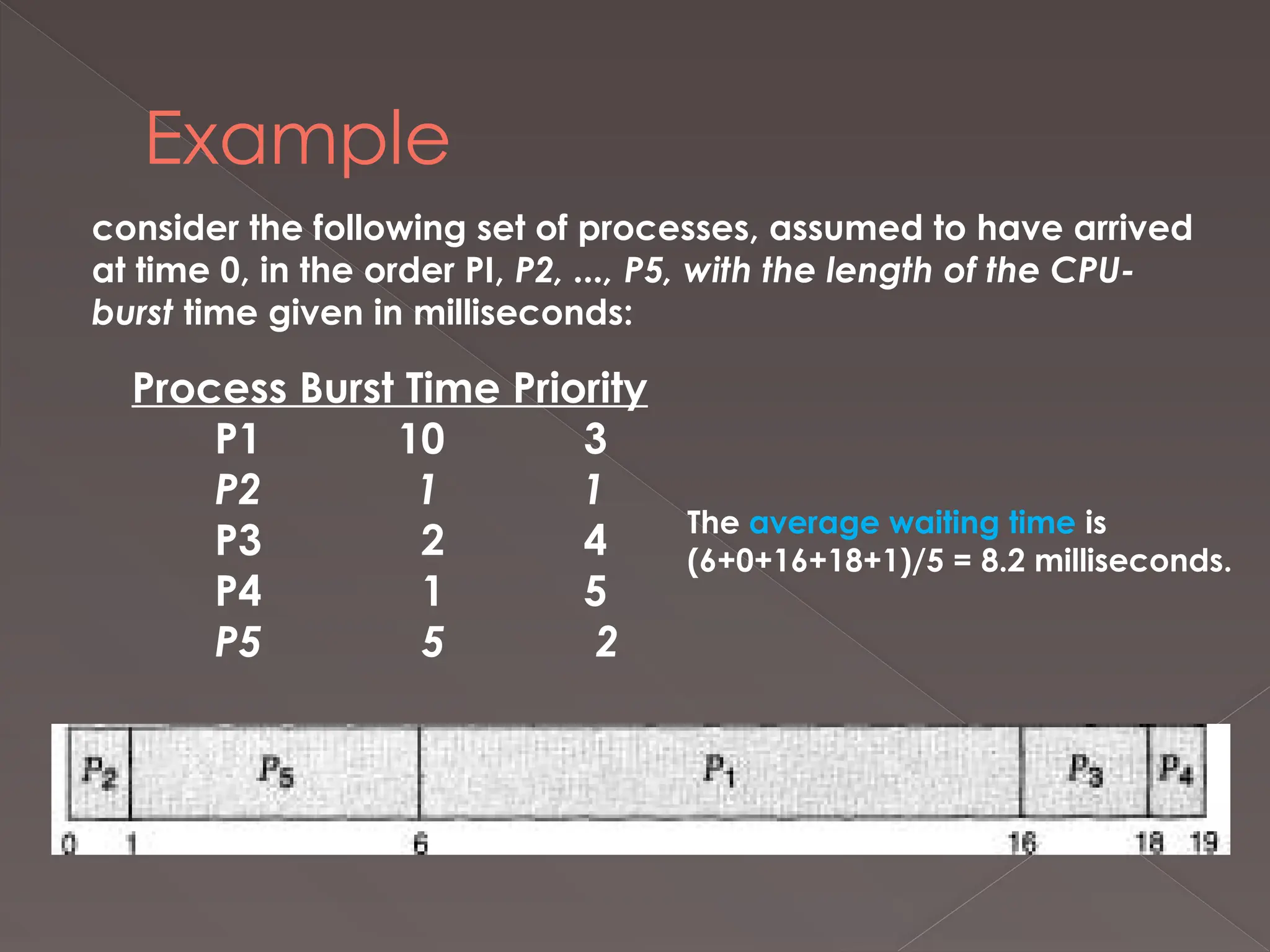
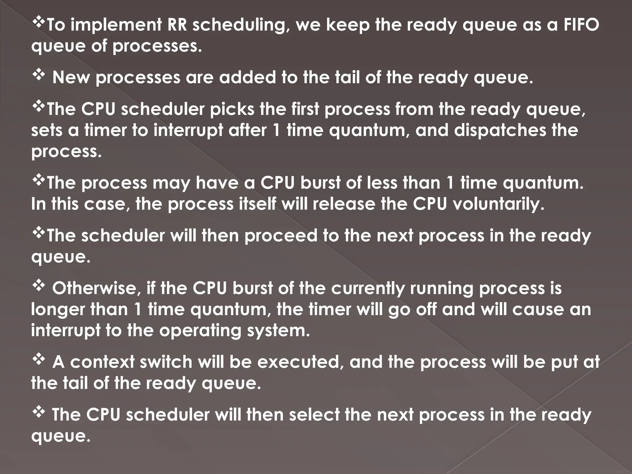
OPERATING SYSTEM
CPU SCHEDULING
BY
MRS.S.RAJAPRIYA,MS(IT).,
ASSISTANT PROFESSOR OF CS
V.V.VANNIAPERUMAL COLLEGE FOR WOMEN,
VIRUDHUNAGAR
CPU-I/O Burst Cycle
The success of CPU scheduling depends on the following observed
property of processes:
Process execution consists of a cycle of CPU execution and I/O
wait. Processes alternate between these two states. Process
execution begins with a CPU burst.
That is followed by an I/O burst, then another CPU burst,
then another I/O burst, and so on.
CPU Scheduler
Whenever the CPU becomes idle, the operating system must
select one of the processes in the ready queue to be executed.
 The selection process is carried out by the short-term scheduler
(or CPU scheduler).
 The scheduler selects from among the processes in memory
that are ready to execute, and allocates the CPU to one of
them.
Preemptive Scheduling
CPU scheduling decisions may take place under the following four
circumstances :
1.When a process switches from the running state to the waiting
state (for example, I/O request, or invocation of wait for the
termination of one of the child processes)
2. When a process switches from the running state to the ready
state (for example, when an interrupt occurs)
3. When a process switches from the waiting state to the ready state
(for example, completion of I/O)
4. When a process terminates In circumstances 1 and 4, there is no
choice in terms of scheduling.
When scheduling takes place only under circumstances 1 and 4,
we say the scheduling scheme is nonpreemptive;
otherwise, the scheduling scheme is preemptive.
Under nonpreemptive scheduling, once the CPU has been
allocated to a process, the process keeps the CPU until it releases the
CPU either by terminating or by switching to the waiting state.
Dispatcher :
Another component involved in the CPU scheduling function is
the dispatcher.
The dispatcher is the module that gives control of the CPU to the
process selected by the short-term scheduler. This function
involves:
1. Switching context
2. Switching to user mode
3. Jumping to the proper location in the user program to restart
that program
The dispatcher should be as fast as possible, given that it is invoked
during every process switch. The time it takes for the dispatcher to
stop one process and start another running is known as the
dispatch latency.
Scheduling Criteria
Many criteria have been suggested for comparing CPU-scheduling
algorithms.
The criteria include the following:
CPU utilization: We want to keep the CPU as busy as possible. CPU
utilization may range from 0 to 100 percent. In a real system, it should
range from 40 percent to 90 percent.
Throughput: If the CPU is busy executing processes, then work is being
done. One measure of work is the number of processes completed
per time unit, called throughput. For long processes, this rate may be
1 process per hour; for short transactions, throughput might be 10
processes per second.
Turnaround time: The interval from the time of submission of a process
to the time of completion is the turnaround time. Turnaround time is
the sum of the periods spent waiting to get into memory, waiting in the
ready queue, executing on the CPU, and doing I/O.
Waiting time: The CPU-scheduling algorithm does not affect the
amount of time during which a process executes or does I/O; it affects
only the amount of time that a process spends waiting in the ready
queue. Waiting time is the sum of the periods spent waiting in the
ready queue.
Response time: It is the time from the submission of a request until the
first response is produced. This measure, called response time, is the
amount of time it takes to start responding, but not the time that it
takes to output that response.
Scheduling Algorithms
CPU scheduling deals with the problem of deciding which of the
processes in the ready queue is to be allocated the CPU. several
of the many CPU-scheduling algorithms that exist.
5.3.1 First-Come, First-Served Scheduling
 The simplest CPU-scheduling algorithm is the first-come, first-
served (FCFS) scheduling algorithm.
With this scheme, the process that requests the CPU first is
allocated the CPU first.
The implementation of the FCFS policy is easily managed with a
FIFO queue.
When a process enters the ready queue, its PCB is linked onto
the tail of the queue.
•When the CPU is free, it is allocated to the process at the head of
the queue.
•The running process is then removed from the queue. The code
for FCFS scheduling is simple to write and understand.
•The average waiting time under the FCFS policy, however, is often
quite long.
FCFS Example
The waiting time is 0
milliseconds for PI, 7
milliseconds for P2,11
milliseconds for P3, and 13
milliseconds for P4.
Average Waiting Time
= (0 + 7 + 11 + 13) / 4
= 7.75 milliseconds
0
7 11 13 18
FCFS Example
Average Response Time
= (0 + 7 + 11 + 13) / 4
= 7.75 milliseconds
(same as Average Waiting
Time)
0
7 11 13 18
FCFS Pros and Cons
•Advantages
– Simple
– Fair (as long as no process hogs the CPU, every
process will eventually run)
• Disadvantages
– Waiting time depends on arrival order
– short processes stuck waiting for long process to
complete
5.3.2 Shortest Job First (SJF)
(no preemption)
•This algorithm associates with each process the length of the
process’s next CPU burst.
•When the CPU is available, it is assigned to the process that has the
smallest next CPU burst.
• If two processes have the same length next CPU burst, FCFS
scheduling is used to break the tie.
Example
consider the following set of processes, with the length of the CPU-burst
time given in milliseconds:
Process Burst Time
PI 6
p2 8
p3 7
p4 3
The waiting time is 3 milliseconds for process PI, 16 milliseconds for
process P2,9 milliseconds for process P3, and 0 milliseconds for
process P4. Thus, the average waiting time is (3 + 16 + 9 + 0)/4 = 7
milliseconds. Average response time= (Average wait time)
Example
Process Completion Time Turn around Time=
C.T – A.T
P1 9 9
P2 24 24
P3 16 16
P4 3 3
•The SJF scheduling algorithm is provably optimal, it gives the
minimum average waiting time for a given set of processes.
• By moving a short process before a long one, the waiting time of
the short process decreases more than it increases the waiting time
of the long process.
•Consequently, the average waiting time decreases.
•Although the SJF algorithm is optimal, it cannot be implemented at
the level of short-term CPU scheduling.
• There is no way to know the length of the next CPU burst.
The next CPU burst is generally predicted as an exponential
average of the measured lengths of previous CPU bursts.
Let t, be the length of the nth
CPU burst, and let be our
predicted value for the next CPU burst. Then, for a, 0 < a < 1,
define
SJF Pros and Cons
•Advantages
– Minimizes average wait time and average response
time
• Disadvantages
– Not practical : difficult to predict burst time
• Learning to predict future
– May starve long jobs
Shortest Remaining Time First
– SRTF (SJF with preemption)
•The SJF algorithm may be either preemptive or non-preemptive.
•The choice arises when a new process arrives at the ready queue
while a previous process is executing.
• The new process may have a shorter next CPU burst than the
currently executing process.
•A preemptive SJF algorithm will preempt the currently executing
process, whereas a non-preemptive SJF algorithm will allow the
currently running process to finish its CPU burst.
• Preemptive SJF scheduling is sometimes called shortest-
remaining-time-first scheduling.
Average wait time
= (7 + 0 + 2 + 1) / 4
= 2.5 millisecond
Response time = Starting
Time – Arrival time
0 1 2 3 4 5 6 7 8 9 14
Priority Scheduling
§A priority is associated with each process, and the CPU is allocated
to the process with the highest priority.
§ Equal-priority processes are scheduled in FCFS order.
§An SJF algorithm is simply a priority algorithm where the priority (p)
is the inverse of the (predicted) next CPU burst.
§ The larger the CPU burst, the lower the priority, and vice versa.
§Priorities are generally some fixed range of numbers, such as 0 to
7, or 0 to 4,095.
§However, there is no general agreement on whether 0 is the
highest or lowest priority.
§ Some systems use low numbers to represent low priority; others
use low numbers for high priority.
Example
consider the following set of processes, assumed to have arrived
at time 0, in the order PI, P2, ..., P5, with the length of the CPU-
burst time given in milliseconds:
Process Burst Time Priority
P1 10 3
P2 1 1
P3 2 4
P4 1 5
P5 5 2
The average waiting time is
(6+0+16+18+1)/5 = 8.2 milliseconds.
Priorities
Priorities can be set internally (by scheduler) or externally (by users)
• Dynamic vs Static
– Static priority : priority of a process is fixed
– Dynamic priority : scheduler can change the process
priority during execution in order to achieve scheduling goals
• eg1. decrease priority of a process to give another process a
chance to execute
• eg.2. increase priority for I/O bound processes
Priority scheduling can be either
preemptive or non-preemptive.
When a process arrives at the ready queue, its priority is
compared with the priority of the currently running process.
A preemptive priority-scheduling algorithm will preempt the
CPU if the priority of the newly arrived process is higher than the
priority of the currently running process.
A non-preemptive priority-scheduling algorithm will simply put
the new process at the head of the ready queue.
Dealing with Starvation
A major problem with priority-scheduling algorithms is indefinite
blocking (or starvation).
A process that is ready to run but lacking the CPU can be
considered blocked-waiting for the CPU.
A priority-scheduling algorithm can leave some low-priority
processes waiting indefinitely for the CPU.
 In a heavily loaded computer system, a steady stream of
higher-priority processes can prevent a low-priority process from
ever getting the CPU.
Solution
A solution to the problem of indefinite blockage of low-priority
processes is aging.
Aging is a technique of gradually increasing the priority of
processes that wait in the system for a long time.
 For example, if priorities range from 127 (low) to 0 (high), we
could decrement the priority of a waiting process by 1 every 15
minutes.
Eventually, even a process with an initial priority of 127 would
have the highest priority in the system and would be executed.
 In fact, it would take no more than 32 hours for a priority 127
process to age to a priority 0 process.
Consider the following processes :
(i)Draw the Grantt chart using preemptive shortest remaining time
first.
(ii) Find the
Round-Robin Scheduling
The round-robin (RR) scheduling algorithm is designed especially
for timesharing systems.
 It is similar to FCFS scheduling, but preemption is added to
switch between processes.
A small unit of time, called a time quantum (or time slice), is
defined.
A time quantum is generally from 10 to 100 milliseconds. The
ready queue is treated as a circular queue.
The CPU scheduler goes around the ready queue, allocating the
CPU to each process for a time interval of up to 1 time quantum.
To implement RR scheduling, we keep the ready queue as a FIFO
queue of processes.
 New processes are added to the tail of the ready queue.
The CPU scheduler picks the first process from the ready queue,
sets a timer to interrupt after 1 time quantum, and dispatches the
process.
The process may have a CPU burst of less than 1 time quantum.
In this case, the process itself will release the CPU voluntarily.
The scheduler will then proceed to the next process in the ready
queue.
 Otherwise, if the CPU burst of the currently running process is
longer than 1 time quantum, the timer will go off and will cause an
interrupt to the operating system.
 A context switch will be executed, and the process will be put at
the tail of the ready queue.
 The CPU scheduler will then select the next process in the ready
queue.
Example
Advantages & Disadvantages
Advantages
– Fair (Each process gets a fair chance to run on the CPU)
– Low average wait time, when burst times vary
– Faster response time
• Disadvantages
– Increased context switching
• Context switches are overheads!!!
– High average wait time, when burst times have equal lengths 20

CPU SCHEDULING ALGORITHMS-FCFS,SJF,RR.pptx

  • 1.
    OPERATING SYSTEM CPU SCHEDULING BY MRS.S.RAJAPRIYA,MS(IT)., ASSISTANTPROFESSOR OF CS V.V.VANNIAPERUMAL COLLEGE FOR WOMEN, VIRUDHUNAGAR
  • 2.
    CPU-I/O Burst Cycle Thesuccess of CPU scheduling depends on the following observed property of processes: Process execution consists of a cycle of CPU execution and I/O wait. Processes alternate between these two states. Process execution begins with a CPU burst. That is followed by an I/O burst, then another CPU burst, then another I/O burst, and so on.
  • 3.
    CPU Scheduler Whenever theCPU becomes idle, the operating system must select one of the processes in the ready queue to be executed.  The selection process is carried out by the short-term scheduler (or CPU scheduler).  The scheduler selects from among the processes in memory that are ready to execute, and allocates the CPU to one of them.
  • 4.
    Preemptive Scheduling CPU schedulingdecisions may take place under the following four circumstances : 1.When a process switches from the running state to the waiting state (for example, I/O request, or invocation of wait for the termination of one of the child processes) 2. When a process switches from the running state to the ready state (for example, when an interrupt occurs) 3. When a process switches from the waiting state to the ready state (for example, completion of I/O) 4. When a process terminates In circumstances 1 and 4, there is no choice in terms of scheduling.
  • 5.
    When scheduling takesplace only under circumstances 1 and 4, we say the scheduling scheme is nonpreemptive; otherwise, the scheduling scheme is preemptive. Under nonpreemptive scheduling, once the CPU has been allocated to a process, the process keeps the CPU until it releases the CPU either by terminating or by switching to the waiting state.
  • 6.
    Dispatcher : Another componentinvolved in the CPU scheduling function is the dispatcher. The dispatcher is the module that gives control of the CPU to the process selected by the short-term scheduler. This function involves: 1. Switching context 2. Switching to user mode 3. Jumping to the proper location in the user program to restart that program The dispatcher should be as fast as possible, given that it is invoked during every process switch. The time it takes for the dispatcher to stop one process and start another running is known as the dispatch latency.
  • 7.
    Scheduling Criteria Many criteriahave been suggested for comparing CPU-scheduling algorithms. The criteria include the following: CPU utilization: We want to keep the CPU as busy as possible. CPU utilization may range from 0 to 100 percent. In a real system, it should range from 40 percent to 90 percent. Throughput: If the CPU is busy executing processes, then work is being done. One measure of work is the number of processes completed per time unit, called throughput. For long processes, this rate may be 1 process per hour; for short transactions, throughput might be 10 processes per second.
  • 8.
    Turnaround time: Theinterval from the time of submission of a process to the time of completion is the turnaround time. Turnaround time is the sum of the periods spent waiting to get into memory, waiting in the ready queue, executing on the CPU, and doing I/O. Waiting time: The CPU-scheduling algorithm does not affect the amount of time during which a process executes or does I/O; it affects only the amount of time that a process spends waiting in the ready queue. Waiting time is the sum of the periods spent waiting in the ready queue. Response time: It is the time from the submission of a request until the first response is produced. This measure, called response time, is the amount of time it takes to start responding, but not the time that it takes to output that response.
  • 9.
    Scheduling Algorithms CPU schedulingdeals with the problem of deciding which of the processes in the ready queue is to be allocated the CPU. several of the many CPU-scheduling algorithms that exist. 5.3.1 First-Come, First-Served Scheduling  The simplest CPU-scheduling algorithm is the first-come, first- served (FCFS) scheduling algorithm. With this scheme, the process that requests the CPU first is allocated the CPU first. The implementation of the FCFS policy is easily managed with a FIFO queue. When a process enters the ready queue, its PCB is linked onto the tail of the queue.
  • 10.
    •When the CPUis free, it is allocated to the process at the head of the queue. •The running process is then removed from the queue. The code for FCFS scheduling is simple to write and understand. •The average waiting time under the FCFS policy, however, is often quite long.
  • 11.
    FCFS Example The waitingtime is 0 milliseconds for PI, 7 milliseconds for P2,11 milliseconds for P3, and 13 milliseconds for P4. Average Waiting Time = (0 + 7 + 11 + 13) / 4 = 7.75 milliseconds 0 7 11 13 18
  • 12.
    FCFS Example Average ResponseTime = (0 + 7 + 11 + 13) / 4 = 7.75 milliseconds (same as Average Waiting Time) 0 7 11 13 18
  • 13.
    FCFS Pros andCons •Advantages – Simple – Fair (as long as no process hogs the CPU, every process will eventually run) • Disadvantages – Waiting time depends on arrival order – short processes stuck waiting for long process to complete
  • 14.
    5.3.2 Shortest JobFirst (SJF) (no preemption) •This algorithm associates with each process the length of the process’s next CPU burst. •When the CPU is available, it is assigned to the process that has the smallest next CPU burst. • If two processes have the same length next CPU burst, FCFS scheduling is used to break the tie.
  • 15.
    Example consider the followingset of processes, with the length of the CPU-burst time given in milliseconds: Process Burst Time PI 6 p2 8 p3 7 p4 3 The waiting time is 3 milliseconds for process PI, 16 milliseconds for process P2,9 milliseconds for process P3, and 0 milliseconds for process P4. Thus, the average waiting time is (3 + 16 + 9 + 0)/4 = 7 milliseconds. Average response time= (Average wait time)
  • 16.
    Example Process Completion TimeTurn around Time= C.T – A.T P1 9 9 P2 24 24 P3 16 16 P4 3 3
  • 17.
    •The SJF schedulingalgorithm is provably optimal, it gives the minimum average waiting time for a given set of processes. • By moving a short process before a long one, the waiting time of the short process decreases more than it increases the waiting time of the long process. •Consequently, the average waiting time decreases. •Although the SJF algorithm is optimal, it cannot be implemented at the level of short-term CPU scheduling. • There is no way to know the length of the next CPU burst.
  • 18.
    The next CPUburst is generally predicted as an exponential average of the measured lengths of previous CPU bursts. Let t, be the length of the nth CPU burst, and let be our predicted value for the next CPU burst. Then, for a, 0 < a < 1, define
  • 19.
    SJF Pros andCons •Advantages – Minimizes average wait time and average response time • Disadvantages – Not practical : difficult to predict burst time • Learning to predict future – May starve long jobs
  • 20.
    Shortest Remaining TimeFirst – SRTF (SJF with preemption) •The SJF algorithm may be either preemptive or non-preemptive. •The choice arises when a new process arrives at the ready queue while a previous process is executing. • The new process may have a shorter next CPU burst than the currently executing process. •A preemptive SJF algorithm will preempt the currently executing process, whereas a non-preemptive SJF algorithm will allow the currently running process to finish its CPU burst. • Preemptive SJF scheduling is sometimes called shortest- remaining-time-first scheduling.
  • 21.
    Average wait time =(7 + 0 + 2 + 1) / 4 = 2.5 millisecond Response time = Starting Time – Arrival time 0 1 2 3 4 5 6 7 8 9 14
  • 22.
    Priority Scheduling §A priorityis associated with each process, and the CPU is allocated to the process with the highest priority. § Equal-priority processes are scheduled in FCFS order. §An SJF algorithm is simply a priority algorithm where the priority (p) is the inverse of the (predicted) next CPU burst. § The larger the CPU burst, the lower the priority, and vice versa. §Priorities are generally some fixed range of numbers, such as 0 to 7, or 0 to 4,095. §However, there is no general agreement on whether 0 is the highest or lowest priority. § Some systems use low numbers to represent low priority; others use low numbers for high priority.
  • 23.
    Example consider the followingset of processes, assumed to have arrived at time 0, in the order PI, P2, ..., P5, with the length of the CPU- burst time given in milliseconds: Process Burst Time Priority P1 10 3 P2 1 1 P3 2 4 P4 1 5 P5 5 2 The average waiting time is (6+0+16+18+1)/5 = 8.2 milliseconds.
  • 24.
    Priorities Priorities can beset internally (by scheduler) or externally (by users) • Dynamic vs Static – Static priority : priority of a process is fixed – Dynamic priority : scheduler can change the process priority during execution in order to achieve scheduling goals • eg1. decrease priority of a process to give another process a chance to execute • eg.2. increase priority for I/O bound processes
  • 25.
    Priority scheduling canbe either preemptive or non-preemptive. When a process arrives at the ready queue, its priority is compared with the priority of the currently running process. A preemptive priority-scheduling algorithm will preempt the CPU if the priority of the newly arrived process is higher than the priority of the currently running process. A non-preemptive priority-scheduling algorithm will simply put the new process at the head of the ready queue.
  • 26.
    Dealing with Starvation Amajor problem with priority-scheduling algorithms is indefinite blocking (or starvation). A process that is ready to run but lacking the CPU can be considered blocked-waiting for the CPU. A priority-scheduling algorithm can leave some low-priority processes waiting indefinitely for the CPU.  In a heavily loaded computer system, a steady stream of higher-priority processes can prevent a low-priority process from ever getting the CPU.
  • 27.
    Solution A solution tothe problem of indefinite blockage of low-priority processes is aging. Aging is a technique of gradually increasing the priority of processes that wait in the system for a long time.  For example, if priorities range from 127 (low) to 0 (high), we could decrement the priority of a waiting process by 1 every 15 minutes. Eventually, even a process with an initial priority of 127 would have the highest priority in the system and would be executed.  In fact, it would take no more than 32 hours for a priority 127 process to age to a priority 0 process.
  • 28.
    Consider the followingprocesses : (i)Draw the Grantt chart using preemptive shortest remaining time first. (ii) Find the
  • 29.
    Round-Robin Scheduling The round-robin(RR) scheduling algorithm is designed especially for timesharing systems.  It is similar to FCFS scheduling, but preemption is added to switch between processes. A small unit of time, called a time quantum (or time slice), is defined. A time quantum is generally from 10 to 100 milliseconds. The ready queue is treated as a circular queue. The CPU scheduler goes around the ready queue, allocating the CPU to each process for a time interval of up to 1 time quantum.
  • 30.
    To implement RRscheduling, we keep the ready queue as a FIFO queue of processes.  New processes are added to the tail of the ready queue. The CPU scheduler picks the first process from the ready queue, sets a timer to interrupt after 1 time quantum, and dispatches the process. The process may have a CPU burst of less than 1 time quantum. In this case, the process itself will release the CPU voluntarily. The scheduler will then proceed to the next process in the ready queue.  Otherwise, if the CPU burst of the currently running process is longer than 1 time quantum, the timer will go off and will cause an interrupt to the operating system.  A context switch will be executed, and the process will be put at the tail of the ready queue.  The CPU scheduler will then select the next process in the ready queue.
  • 31.
  • 33.
    Advantages & Disadvantages Advantages –Fair (Each process gets a fair chance to run on the CPU) – Low average wait time, when burst times vary – Faster response time • Disadvantages – Increased context switching • Context switches are overheads!!! – High average wait time, when burst times have equal lengths 20