Downloaded 358 times

This document discusses various concepts and algorithms related to process scheduling. It covers basic concepts like CPU bursts and scheduling criteria. It then describes several common scheduling algorithms like FCFS, SJF, priority scheduling, and round robin. It also discusses more advanced topics like multiple processor scheduling, thread scheduling, and load balancing.
Introduction to process scheduling, its basic concepts, criteria, algorithms, and thread scheduling.
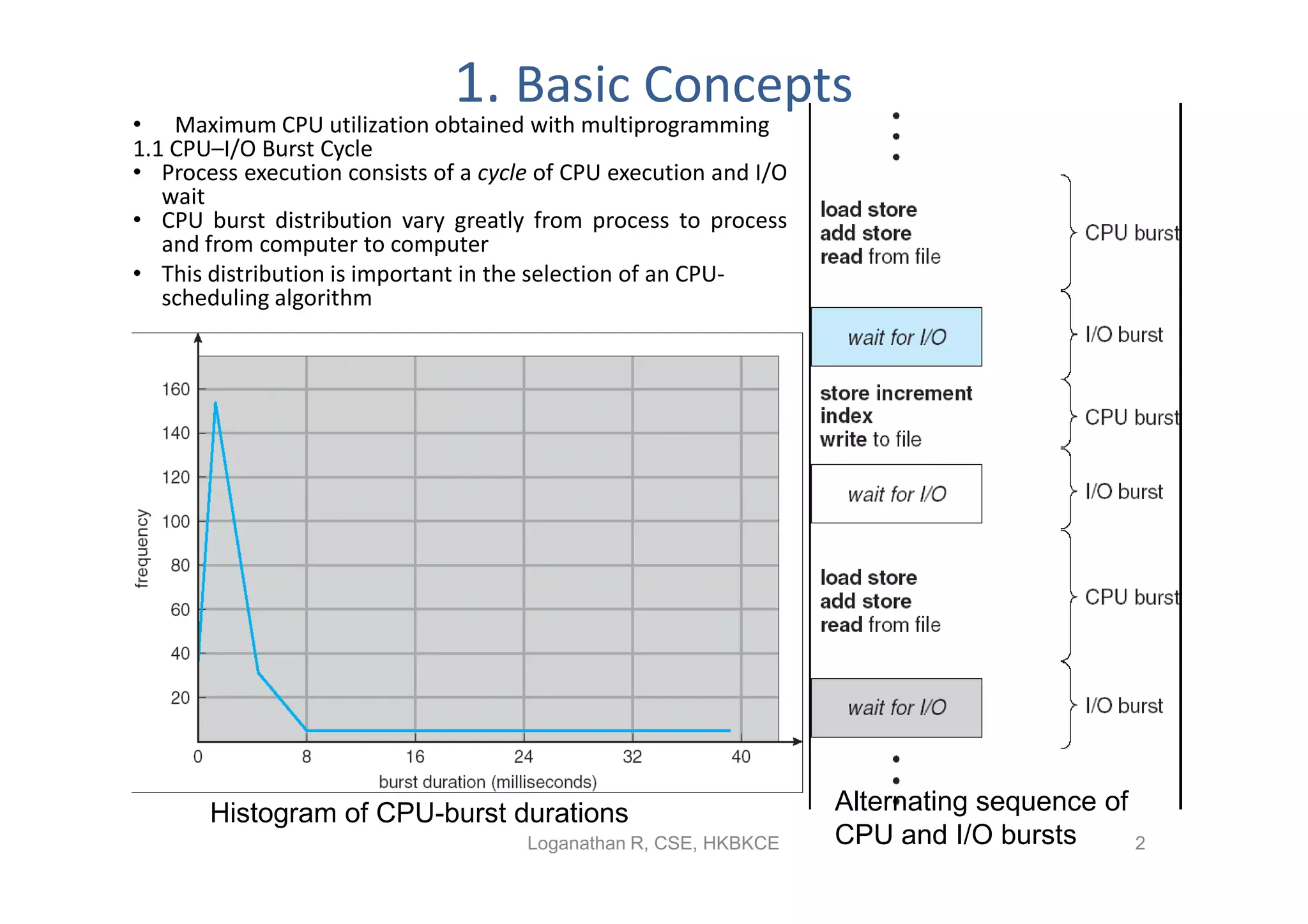
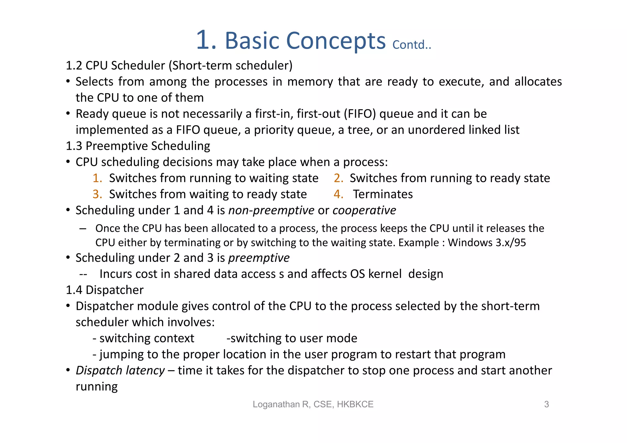
Details process execution with CPU-I/O burst cycles, role of CPU scheduler, dispatcher, and preemptive scheduling concepts.
Outlines scheduling criteria such as CPU utilization, throughput, turnaround time, waiting time, and response time.
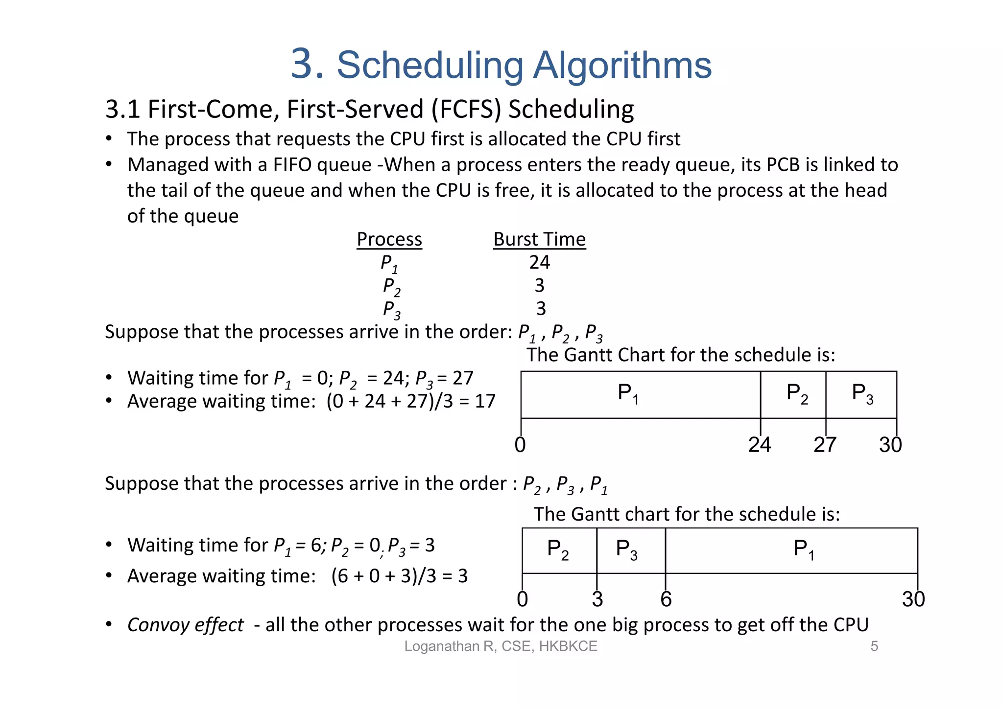
Explanation of FCFS scheduling with examples, waiting time calculations, and introduction to convoy effect.
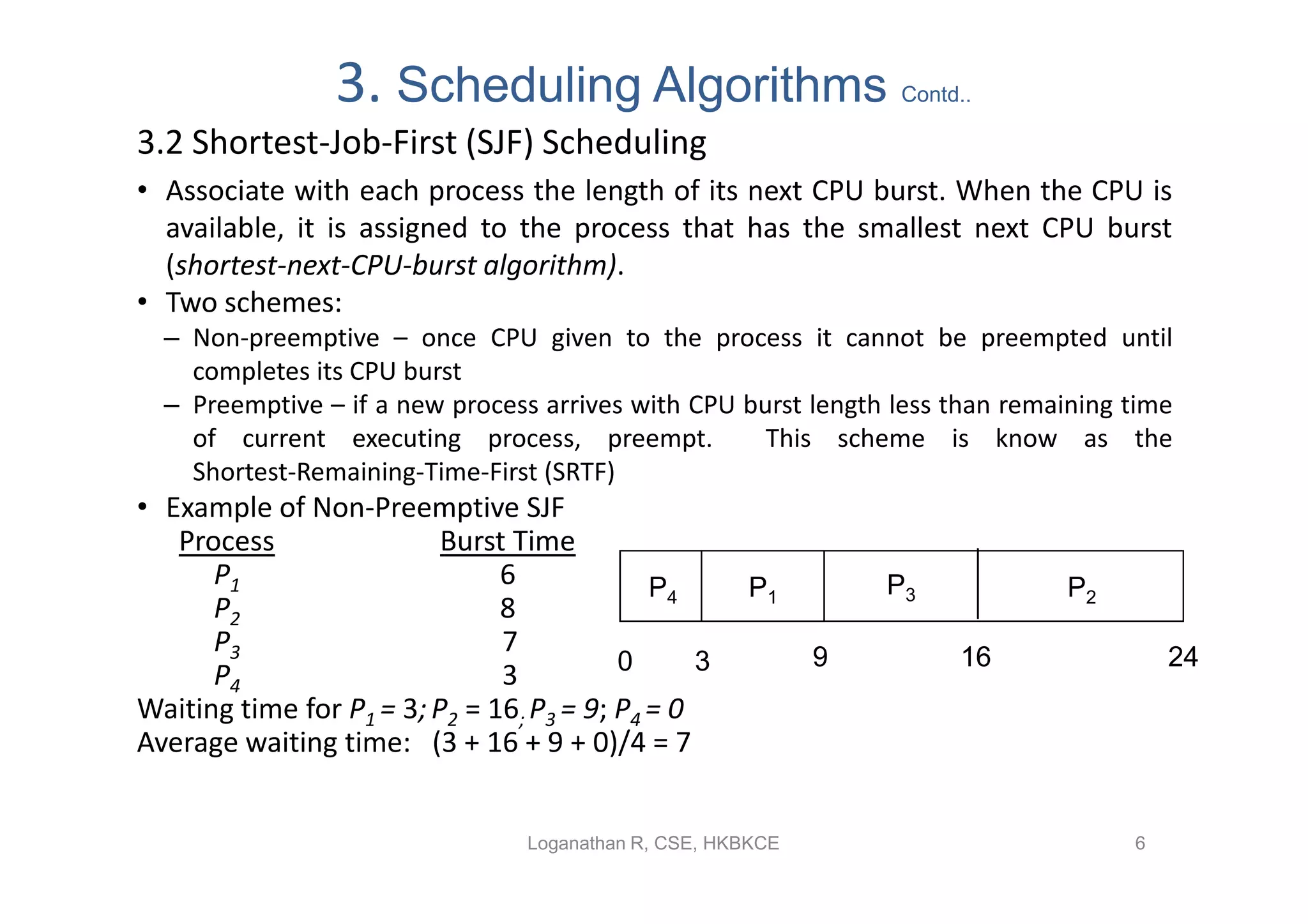
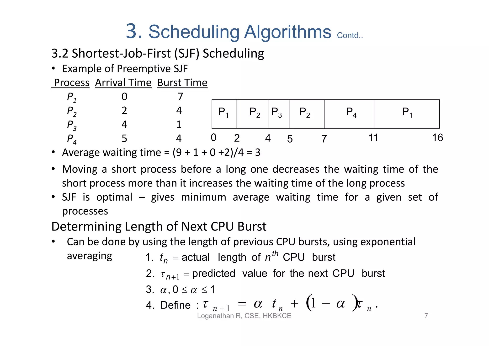
Discusses non-preemptive and preemptive SJF scheduling with examples and average waiting time calculations.
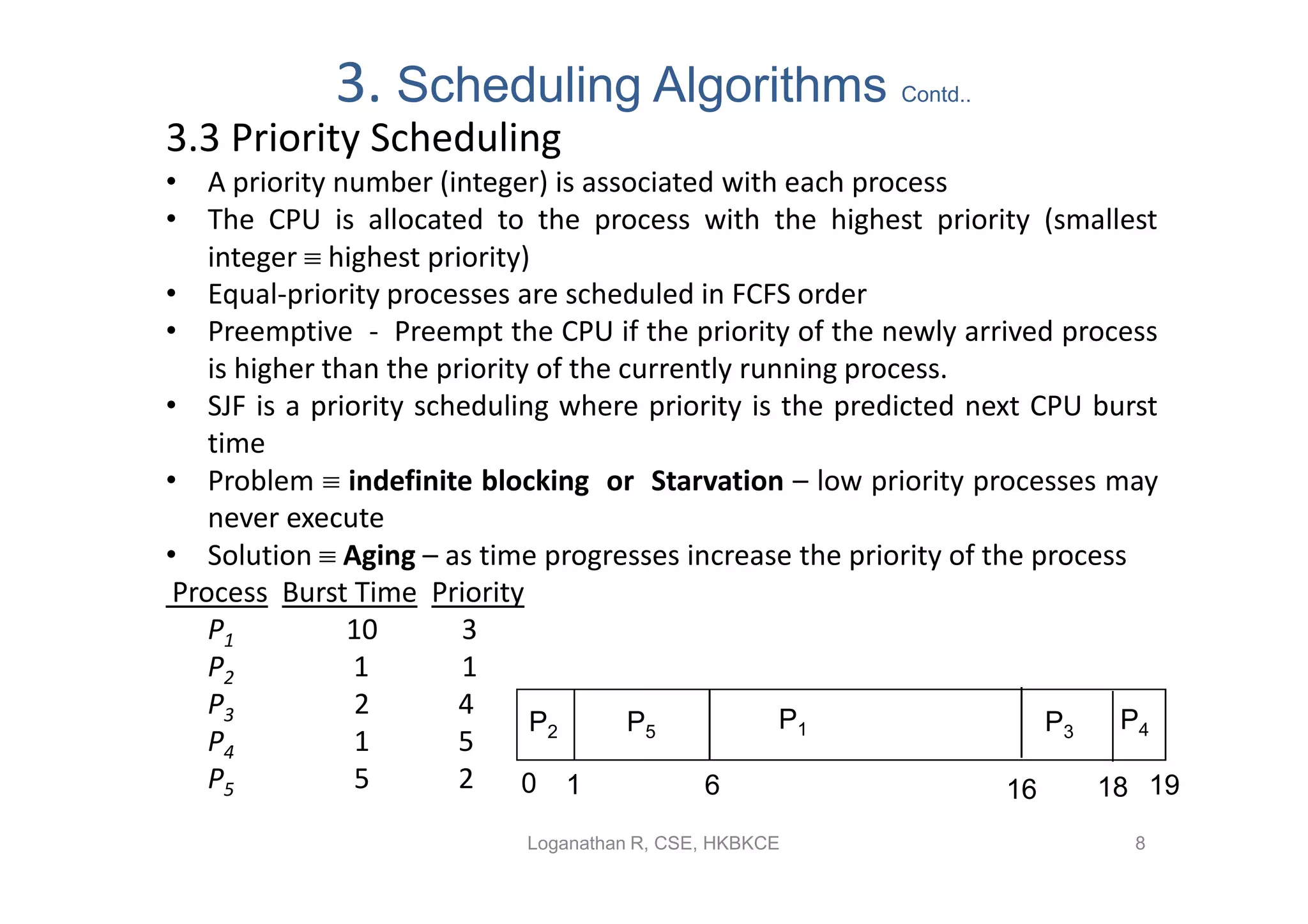
Overview of priority scheduling, including problems like starvation and solutions such as aging.
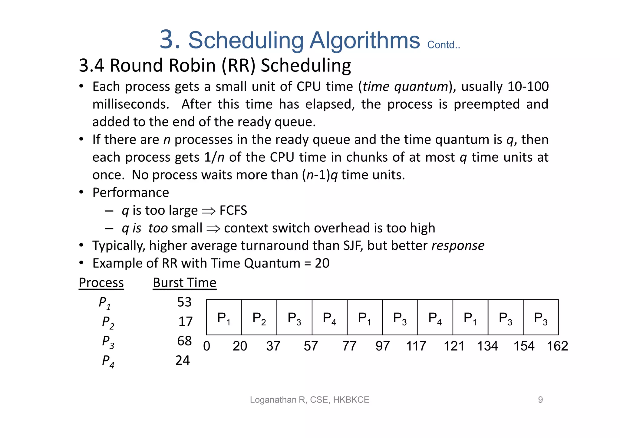
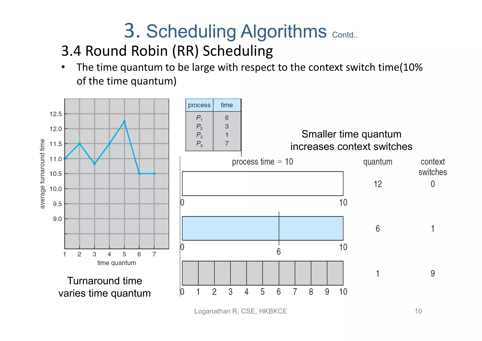
Describes round robin scheduling, time quantum effects, and performance implications on turnaround time.
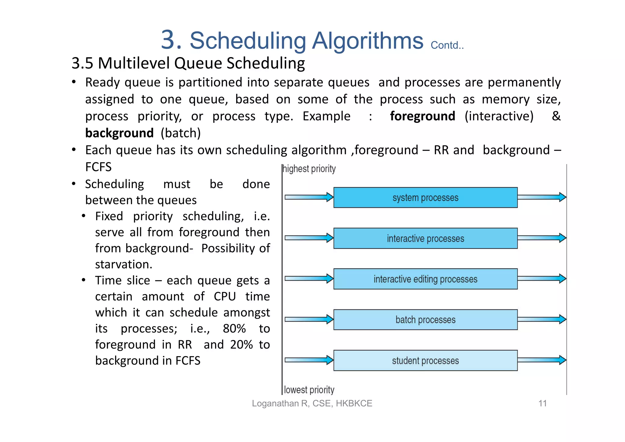
Explains multilevel queue scheduling, allocation of processes to queues, and scheduling strategies.
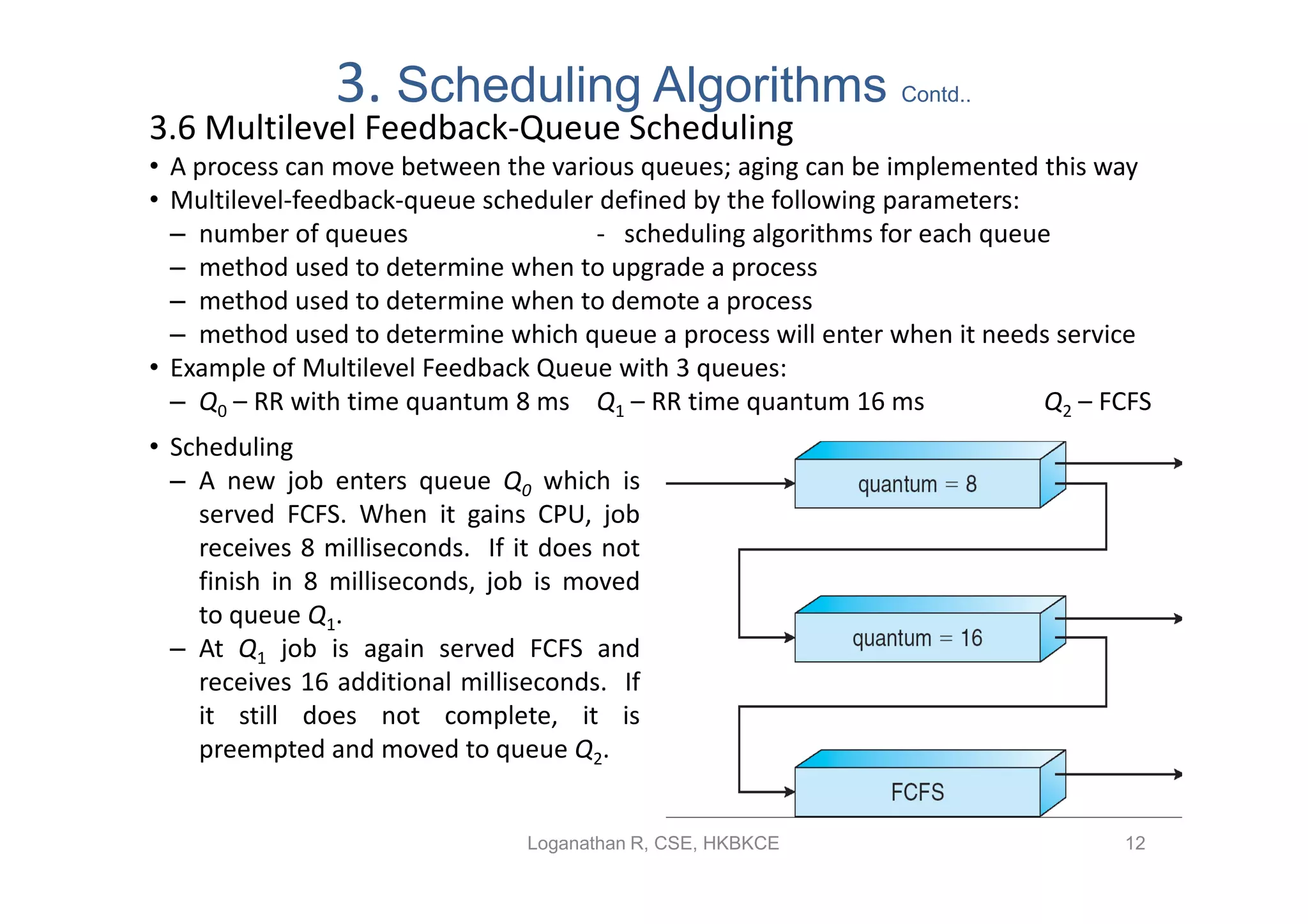
Outlines multilevel feedback-queue scheduling, process movement between queues and scheduling parameters.
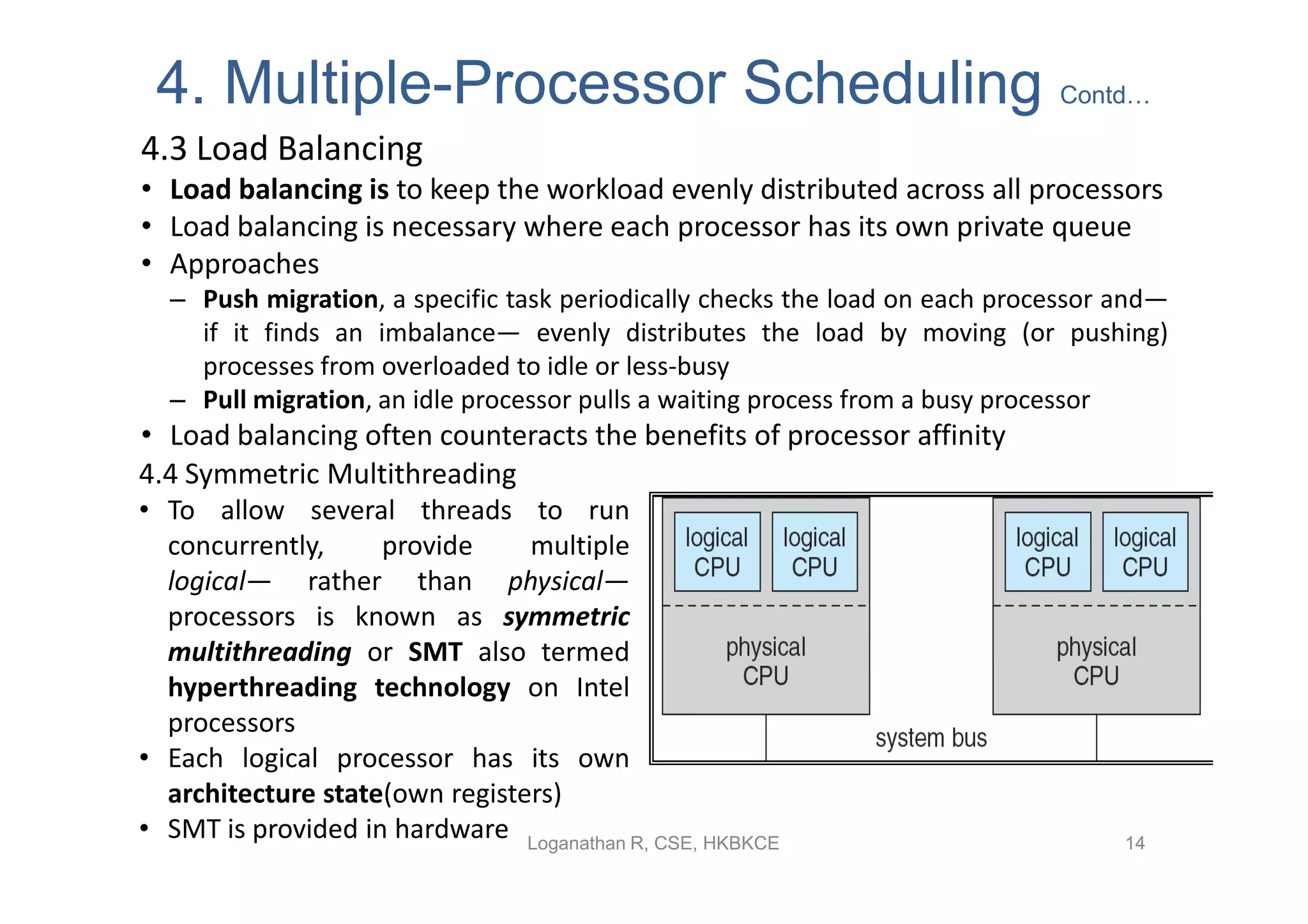
Discusses complexities of CPU scheduling in multiprocessor systems, approaches like SMP, and load balancing.
Examines thread scheduling issues, user-level vs kernel-level threads, and contention scope.