lklhtrlihtro

1. CPU Scheduling

2. CHAPTER OBJECTIVES
• To introduce CPU scheduling, which is the basis for multiprogrammed
operating systems.
• To describe various CPU-scheduling algorithms.
• To discuss evaluation criteria for selecting a CPU-scheduling algorithm
for a particular system.
• To examine the scheduling algorithms of several operating systems.

3. Basic Concepts
CPU scheduling is a process of allocating the CPU to a process or
thread from a pool of ready to run process or thread.
Main Goals are:
●
Maximize CPU utlization
●
Minimize response time
●
Ensure faireness and priority
●
Optimize throughput

4. CPU – I/O Burst Cycle
●
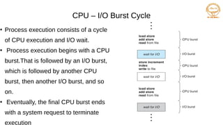
Process execution consists of a cycle
of CPU execution and I/O wait.
●
Process execution begins with a CPU
burst.That is followed by an I/O burst,
which is followed by another CPU
burst, then another I/O burst, and so
on.
●
Eventually, the final CPU burst ends
with a system request to terminate
execution

5. CPU Scheduler
●
Short-term scheduler selects from among the processes in ready queue, and
allocates the CPU to one of them
Queue may be ordered in various ways
●
CPU scheduling decisions may take place when a process:
1. Switches from running to waiting state
2. Switches from running to ready state
3. Switches from waiting to ready
4.Terminates
●
Scheduling under 1 and 4 is nonpreemptive
●
All other scheduling is preemptive
Consider access to shared data
Consider preemption while in kernel mode
Consider interrupts occurring during crucial OS activities

6. Dispatcher
●
Dispatcher module gives control of the CPU to the process selected by
the short-term scheduler; this involves:
switching context
switching to user mode
jumping to the proper location in the user program to restart that
program
●
Dispatch latency – time it takes for the dispatcher to stop one process
and start another running

7. ●
CPU utilization – keep the CPU as busy as possible
●
Throughput – Number of processes that complete their execution per time unit.
●
Turnaround time-The interval from the time of submission of a process to the
time of completion (how long it takes to execute that process.) .Periods spent
waiting to get into memory + waiting in the ready queue + executing on the CPU
+ and doing I/O.
●
Waiting time – amount of time a process has been waiting in the ready queue
●
Response time – amount of time it takes from when a request was submitted
until the first response is produced, not output (for time-sharing environment)
Scheduling Criteria

8. Scheduling Algorithm Optimization Criteria
●
Max CPU utilization
●
Max throughput
●
Min turnaround time
●
Min waiting time
●
Min response time

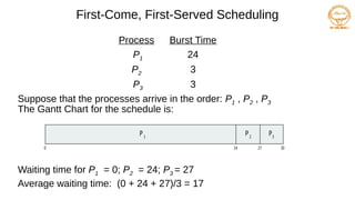
9. First-Come, First-Served Scheduling
Process Burst Time
P1 24
P2 3
P3 3
Suppose that the processes arrive in the order: P1 , P2 , P3
The Gantt Chart for the schedule is:
Waiting time for P1 = 0; P2 = 24; P3 = 27
Average waiting time: (0 + 24 + 27)/3 = 17
P P P
1 2 3
0 24 30
27

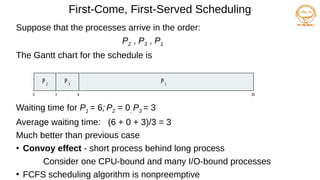
10. First-Come, First-Served Scheduling
Suppose that the processes arrive in the order:
P2 , P3 , P1
The Gantt chart for the schedule is
Waiting time for P1 = 6; P2 = 0; P3 = 3
Average waiting time: (6 + 0 + 3)/3 = 3
Much better than previous case
●
Convoy effect - short process behind long process
Consider one CPU-bound and many I/O-bound processes
●
FCFS scheduling algorithm is nonpreemptive
P1
0 3 6 30
P2
P3

11. Shortest-Job-First (SJF) Scheduling
●
Associate with each process the length of its next CPU burst
Use these lengths to schedule the process with the shortest time
●
SJF is optimal – gives minimum average waiting time for a given set of
processes
The difficulty is knowing the length of the next CPU request
Could ask the user

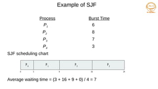
12. Example of SJF
ProcessArriva l TimeBurst Time
P1 0.0 6
P2 2.0 8
P3 4.0 7
P4 5.0 3
SJF scheduling chart
Average waiting time = (3 + 16 + 9 + 0) / 4 = 7
P3
0 3 24
P4
P1
16
9
P2

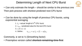
13. Determining Length of Next CPU Burst
●
Can only estimate the length – should be similar to the previous one
Then pick process with shortest predicted next CPU burst
●
Can be done by using the length of previous CPU bursts, using
exponential averaging
Commonly, α set to ½ (Smoothing factor)
●
Preemptive version called shortest-remaining-time-first
:
Define
4.
1
0
,
3.
burst
CPU
next
the
for
value
predicted
2.
burst
CPU
of
length
actual
1.







 1
n
th
n n
t

14. Example of Shortest-remaining-time-first
Now we add the concepts of varying arrival times and preemption to the
analysis
ProcessAarri Arrival TimeTBurst Time
P1 0 8
P2 1 4
P3 2 9
P4 3 5
Preemptive SJF Gantt Chart
Average waiting time = [(10-1)+(1-1)+(17-2)+5-3)]/4 = 26/4 = 6.5 msec
P4
0 1 26
P1
P2
10
P3
P1
5 17

15. Priority Scheduling
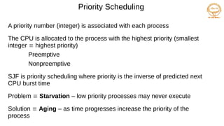
A priority number (integer) is associated with each process
The CPU is allocated to the process with the highest priority (smallest
integer  highest priority)
Preemptive
Nonpreemptive
SJF is priority scheduling where priority is the inverse of predicted next
CPU burst time
Problem  Starvation – low priority processes may never execute
Solution  Aging – as time progresses increase the priority of the
process

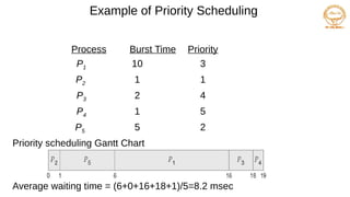
16. Example of Priority Scheduling
ProcessAarri Burst TimeT Priority
P1 10 3
P2 1 1
P3 2 4
P4 1 5
P5 5 2
Priority scheduling Gantt Chart
Average waiting time = (6+0+16+18+1)/5=8.2 msec

17. Round Robin (RR)
●
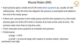
Each process gets a small unit of CPU time (time quantum q), usually 10-100
milliseconds. After this time has elapsed, the process is preempted and added to
the end of the ready queue.
●
If there are n processes in the ready queue and the time quantum is q, then each
process gets 1/n of the CPU time in chunks of at most q time units at once. No
process waits more than (n-1)q time units.
●
Timer interrupts every quantum to schedule next process
●
Performance
q large  FIFO
q small  q must be large with respect to context switch, otherwise
overhead is too high

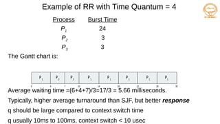
18. Example of RR with Time Quantum = 4
Process Burst Time
P1 24
P2 3
P3 3
The Gantt chart is:
Average waiting time =(6+4+7)/3=17/3 = 5.66 milliseconds.
Typically, higher average turnaround than SJF, but better response
q should be large compared to context switch time
q usually 10ms to 100ms, context switch < 10 usec
P P P
1 1 1
0 18 30
26
14
4 7 10 22
P2
P3
P1
P1
P1

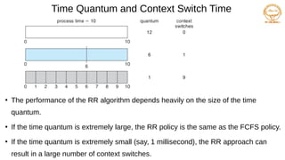
19. Time Quantum and Context Switch Time
●
The performance of the RR algorithm depends heavily on the size of the time
quantum.
●
If the time quantum is extremely large, the RR policy is the same as the FCFS policy.
●
If the time quantum is extremely small (say, 1 millisecond), the RR approach can
result in a large number of context switches.

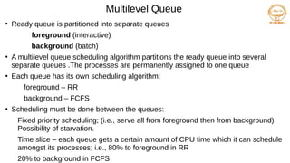
20. Multilevel Queue
●
Ready queue is partitioned into separate queues
foreground (interactive)
background (batch)
●
A multilevel queue scheduling algorithm partitions the ready queue into several
separate queues .The processes are permanently assigned to one queue
●
Each queue has its own scheduling algorithm:
foreground – RR
background – FCFS
●
Scheduling must be done between the queues:
Fixed priority scheduling; (i.e., serve all from foreground then from background).
Possibility of starvation.
Time slice – each queue gets a certain amount of CPU time which it can schedule
amongst its processes; i.e., 80% to foreground in RR
20% to background in FCFS

21. Multilevel Queue Scheduling

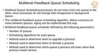
22. Multilevel Feedback Queue Scheduling
●
Multilevel Queue Scheduling processes do not move from one queue to the
other, since processes do not change their foreground or background
nature.
●
The multilevel feedback queue scheduling algorithm, allows a process to
move between queues. Aging can be implemented this way
●
Multilevel-feedback-queue scheduler defined by the following parameters:

Number of queues

Scheduling algorithms for each queue

Method used to determine when to upgrade a process

Method used to determine when to demote a process

Method used to determine which queue a process will enter when that
process needs service

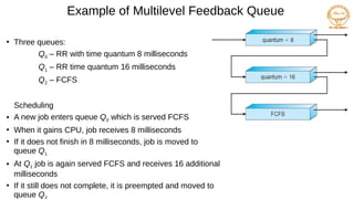
23. Example of Multilevel Feedback Queue
●
Three queues:
Q0 – RR with time quantum 8 milliseconds
Q1 – RR time quantum 16 milliseconds
Q2 – FCFS
Scheduling
● A new job enters queue Q0 which is served FCFS
●
When it gains CPU, job receives 8 milliseconds
●
If it does not finish in 8 milliseconds, job is moved to
queue Q1
● At Q1 job is again served FCFS and receives 16 additional
milliseconds
●
If it still does not complete, it is preempted and moved to
queue Q

24. Thread Scheduling
●
In kernel-level threads—not processes—that are being scheduled by
the operating system.
●
User-level threads are managed by a thread library, and the kernel is
unaware of them.
●
Many-to-one and many-to-many models, thread library schedules user-level
threads to run on LWP

Known as process-contention scope (PCS) since scheduling competition
is within the process

Typically done via priority set by programmer
●
Kernel thread scheduled onto available CPU is system-contention scope
(SCS) – competition among all threads in system

25. Pthread Scheduling
API allows specifying either PCS or SCS during thread creation
PTHREAD_SCOPE_PROCESS schedules threads using PCS scheduling
PTHREAD_SCOPE_SYSTEM schedules threads using SCS scheduling
●
In many-to-many model, the PTHREAD SCOPE PROCESS policy schedules user-
level threads onto available LWPs.
●
The PTHREAD SCOPE SYSTEM scheduling policy will create and bind an LWP for
each user-level thread on many-to-many systems
●
Can be limited by OS – Linux and Mac OS X only allow
PTHREAD_SCOPE_SYSTEM

26. Multiple-Processor Scheduling
●
CPU scheduling more complex when multiple CPUs are available
●
Homogeneous processors within a multiprocessor
●
Asymmetric multiprocessing – only one processor accesses the
system data structures, alleviating the need for data sharing
●
Symmetric multiprocessing (SMP) – each processor is self-
scheduling, all processes in common ready queue, or each has its own
private queue of ready processes

Currently, most common

27. Processor Affinity
●
It refers to the association of a process or thread with specific processor or
core. This technique allows the operating system to optimize process
scheduling ,improve performance and reduce overhead.
●
Hard affinity: permanent binding of a process to a specific processor.
●
Soft affinity :preferences for a process to run on a specific processor but
not guaranteed.

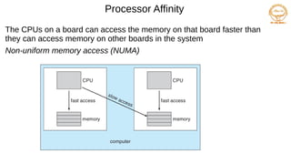
28. Processor Affinity
The CPUs on a board can access the memory on that board faster than
they can access memory on other boards in the system
Non-uniform memory access (NUMA)

29. Multiple-Processor Scheduling
●
If SMP, need to keep all CPUs loaded for efficiency
●
Load balancing attempts to keep the workload evenly distributed
across all processors in an SMP system.
●
There are two general approaches to load balancing: push migration
and pull migration
●
Push migration – periodic task checks load on each processor, and if
found - pushes task from overloaded CPU to other CPUs
●
Pull migration occurs when an idle processor pulls a waiting task from a
busy processor.

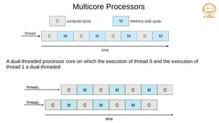
30. Multicore Processors
●
Multicore Processors-Recent trend to place multiple processor cores on same
physical chip
●
Faster and consumes less power
●
Multiple threads per core also growing
Takes advantage of memory stall to make progress on another thread
while memory retrieve happens
when a processor accesses memory, it spends a significant amount of time waiting for the data
to become available. This situation, known as a memory stall

31. Multicore Processors
A dual-threaded processor core on which the execution of thread 0 and the execution of
thread 1 a dual-threaded

32. Real-Time CPU Scheduling
●
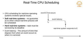
CPU scheduling for real-time operating
systems involves special issues.
●
Soft real-time systems – no guarantee
as to when critical real-time process will
be scheduled
●
Hard real-time systems – task must be
serviced by its deadline
●
Event latency - The amount of time that
elapses from when an event occurs to
when it is serviced

33. Real-Time CPU Scheduling
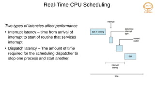
Two types of latencies affect performance
●
Interrupt latency – time from arrival of
interrupt to start of routine that services
interrupt
●
Dispatch latency – The amount of time
required for the scheduling dispatcher to
stop one process and start another.

34. Dispatch latency
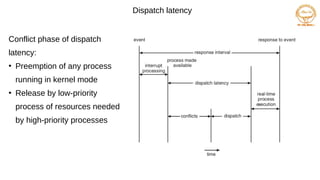
Conflict phase of dispatch
latency:
●
Preemption of any process
running in kernel mode
●
Release by low-priority
process of resources needed
by high-priority processes

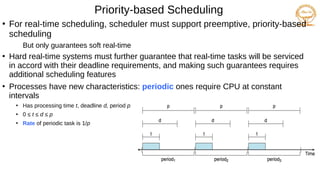
35. Priority-based Scheduling
●
For real-time scheduling, scheduler must support preemptive, priority-based
scheduling
But only guarantees soft real-time
●
Hard real-time systems must further guarantee that real-time tasks will be serviced
in accord with their deadline requirements, and making such guarantees requires
additional scheduling features
●
Processes have new characteristics: periodic ones require CPU at constant
intervals
●
Has processing time t, deadline d, period p
●
0 ≤ t ≤ d ≤ p
●
Rate of periodic task is 1/p

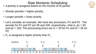
36. Rate Montonic Scheduling
●
A priority is assigned based on the inverse of its period
●
Shorter periods = higher priority;
●
Longer periods = lower priority
●
Let’s consider an example. We have two processes, P1 and P2 . The
periods for P1 and P2 are 50 and 100, respectively—that is, p1 = 50
and p2 = 100. The processing times are t1 = 20 for P1 and t2 = 35 for
P2
● P1 is assigned a higher priority than P2.

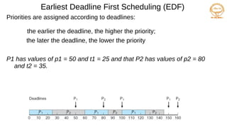
37. Earliest Deadline First Scheduling (EDF)
Priorities are assigned according to deadlines:
the earlier the deadline, the higher the priority;
the later the deadline, the lower the priority
P1 has values of p1 = 50 and t1 = 25 and that P2 has values of p2 = 80
and t2 = 35.

38. Proportional Share Scheduling
T shares are allocated among all processes in the system
An application receives N shares where N < T
This ensures each application will receive N / T of the total processor
time

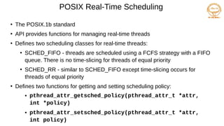
39. POSIX Real-Time Scheduling
●
The POSIX.1b standard
●
API provides functions for managing real-time threads
●
Defines two scheduling classes for real-time threads:
●
SCHED_FIFO - threads are scheduled using a FCFS strategy with a FIFO
queue. There is no time-slicing for threads of equal priority
●
SCHED_RR - similar to SCHED_FIFO except time-slicing occurs for
threads of equal priority
●
Defines two functions for getting and setting scheduling policy:
● pthread_attr_getsched_policy(pthread_attr_t *attr,
int *policy)
● pthread_attr_setsched_policy(pthread_attr_t *attr,
int policy)

40. Operating System Examples
Linux scheduling
Windows scheduling
Solaris scheduling

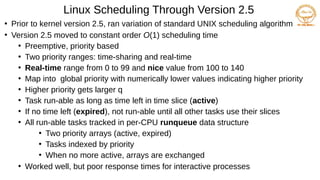
41. Linux Scheduling Through Version 2.5
●
Prior to kernel version 2.5, ran variation of standard UNIX scheduling algorithm
●
Version 2.5 moved to constant order O(1) scheduling time
●
Preemptive, priority based
●
Two priority ranges: time-sharing and real-time
●
Real-time range from 0 to 99 and nice value from 100 to 140
●
Map into global priority with numerically lower values indicating higher priority
●
Higher priority gets larger q
●
Task run-able as long as time left in time slice (active)
●
If no time left (expired), not run-able until all other tasks use their slices
●
All run-able tasks tracked in per-CPU runqueue data structure
●
Two priority arrays (active, expired)
●
Tasks indexed by priority
●
When no more active, arrays are exchanged
●
Worked well, but poor response times for interactive processes

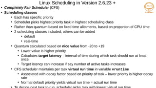
42. Linux Scheduling in Version 2.6.23 +
●
Completely Fair Scheduler (CFS)
●
Scheduling classes
●
Each has specific priority
●
Scheduler picks highest priority task in highest scheduling class
●
Rather than quantum based on fixed time allotments, based on proportion of CPU time
●
2 scheduling classes included, others can be added
●
default
●
real-time
●
Quantum calculated based on nice value from -20 to +19
●
Lower value is higher priority
●
Calculates target latency – interval of time during which task should run at least
once
●
Target latency can increase if say number of active tasks increases
●
CFS scheduler maintains per task virtual run time in variable vruntime
●
Associated with decay factor based on priority of task – lower priority is higher decay
rate
●
Normal default priority yields virtual run time = actual run time
●

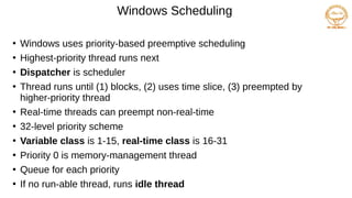
43. Windows Scheduling
●
Windows uses priority-based preemptive scheduling
●
Highest-priority thread runs next
●
Dispatcher is scheduler
●
Thread runs until (1) blocks, (2) uses time slice, (3) preempted by
higher-priority thread
●
Real-time threads can preempt non-real-time
●
32-level priority scheme
●
Variable class is 1-15, real-time class is 16-31
●
Priority 0 is memory-management thread
●
Queue for each priority
●
If no run-able thread, runs idle thread

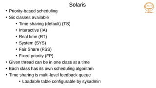
44. Solaris
●
Priority-based scheduling
●
Six classes available
●
Time sharing (default) (TS)
●
Interactive (IA)
●
Real time (RT)
●
System (SYS)
●
Fair Share (FSS)
●
Fixed priority (FP)
●
Given thread can be in one class at a time
●
Each class has its own scheduling algorithm
●
Time sharing is multi-level feedback queue
●
Loadable table configurable by sysadmin

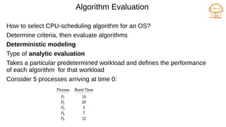
45. Algorithm Evaluation
How to select CPU-scheduling algorithm for an OS?
Determine criteria, then evaluate algorithms
Deterministic modeling
Type of analytic evaluation
Takes a particular predetermined workload and defines the performance
of each algorithm for that workload
Consider 5 processes arriving at time 0:

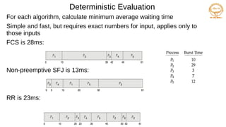
46. Deterministic Evaluation
For each algorithm, calculate minimum average waiting time
Simple and fast, but requires exact numbers for input, applies only to
those inputs
FCS is 28ms:
Non-preemptive SFJ is 13ms:
RR is 23ms: