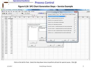
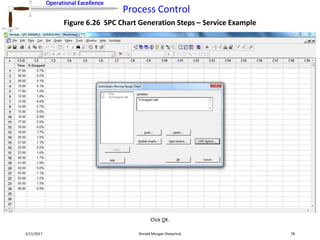
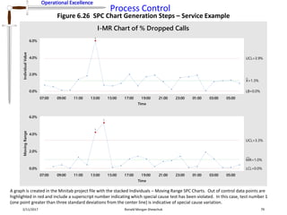
Downloaded 152 times

![Operational Excellence
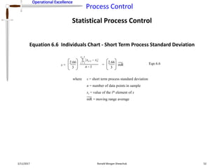
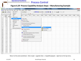
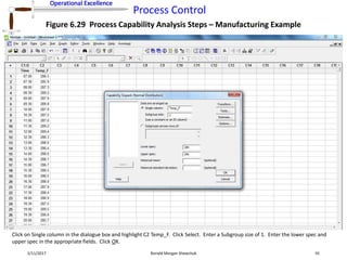
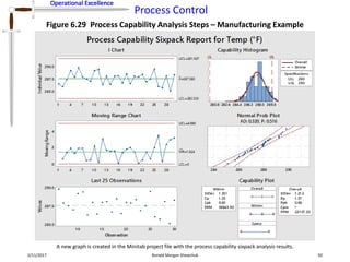
Process Control
Operational Excellence
2/11/2017 Ronald Morgan Shewchuk 34
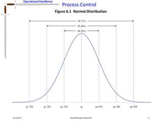
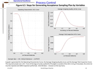
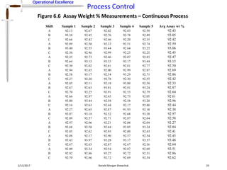
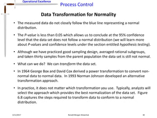
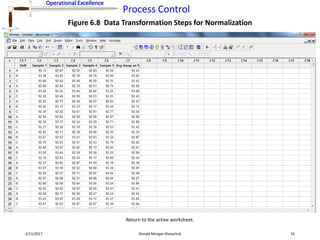
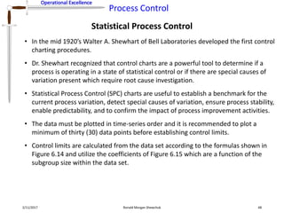
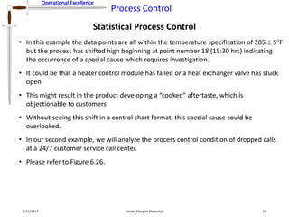
Figure 6.8 Data Transformation Steps for Normalization
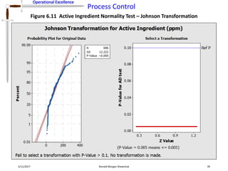
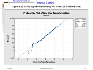
The Johnson Transformation probability plot is created in the Minitab project file. The transformation was successful to normalize the data set.
The transformed data has a P-value which is well above 0.05. The derived transformation function is given as
1.35408 + 1.07249 * ln[(X - 92.2172)/(93.9892 - X)] where X is the original average assay wt% variable.](https://image.slidesharecdn.com/processcontrol-170211173936/85/Process-Control-34-320.jpg)


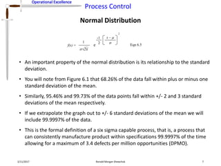
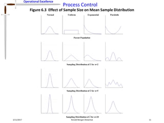
This document discusses process control and operational excellence. It covers key topics like: - Reducing variation is important for process control and profitability. Variation is the enemy of Six Sigma. - Standard deviation and variance are statistical measures of variation. Standard deviation quantifies how far data points deviate from the mean on average. Variance is the square of standard deviation. - Many processes follow a normal distribution curve. Six sigma quality implies processes operate within 6 standard deviations of the mean 99.9997% of the time. - Effective sampling plan design is needed to ensure sample data represents the true population and allows for statistical analysis despite non-normal parent distributions, according to the central limit theorem.


![Process Capability[1]](https://cdn.slidesharecdn.com/ss_thumbnails/processcapability1-1226090261326164-9-thumbnail.jpg?width=640&height=640&fit=bounds)