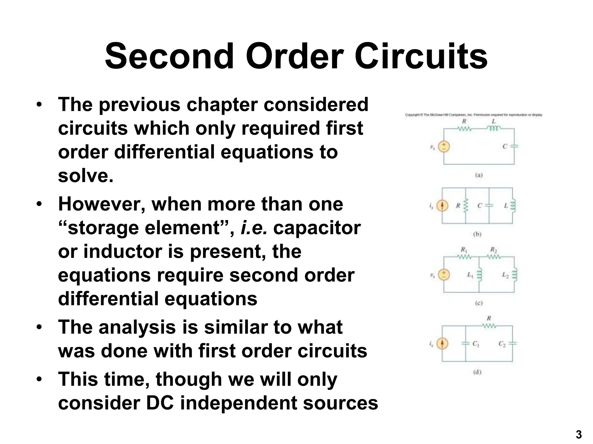
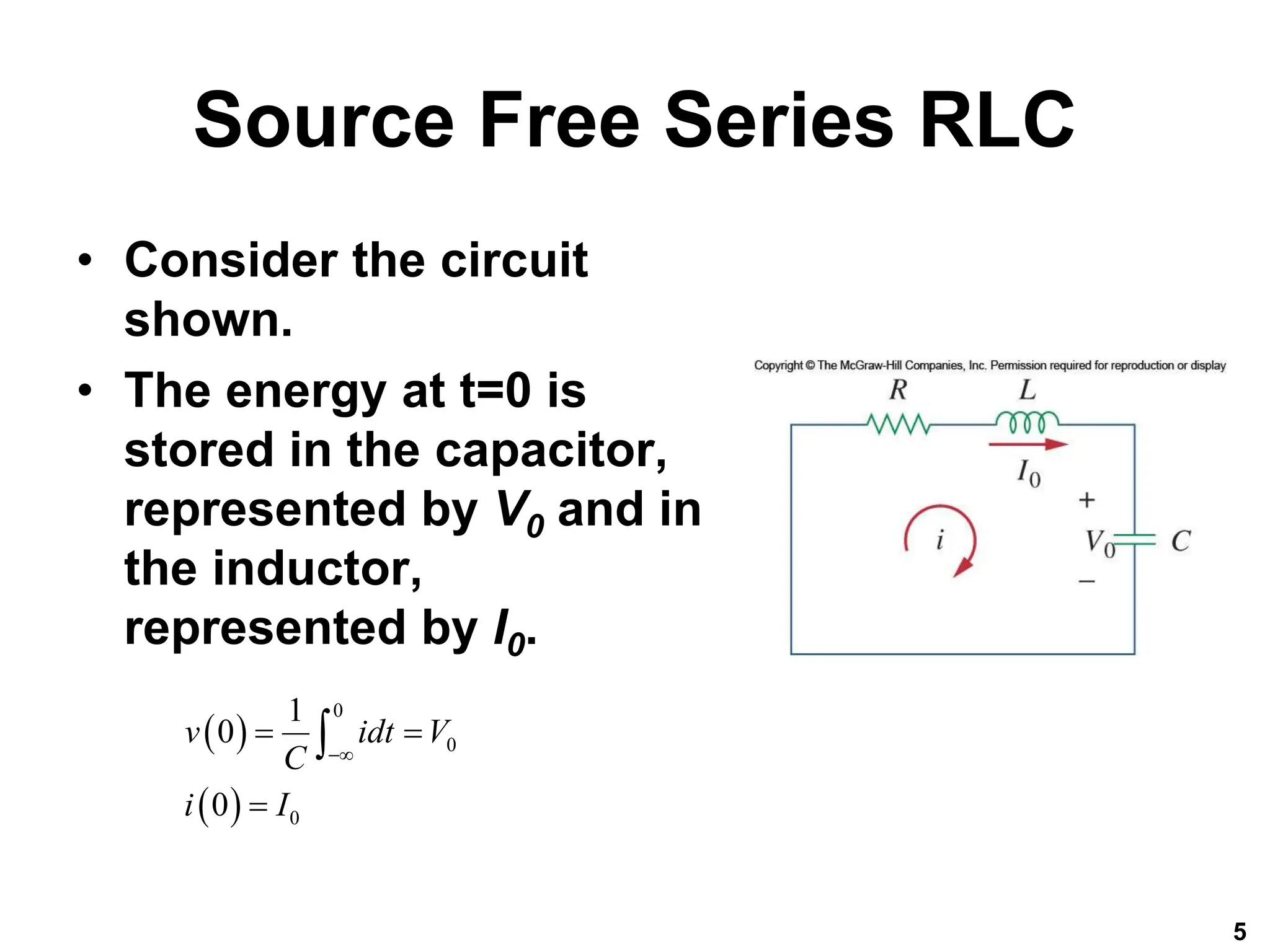
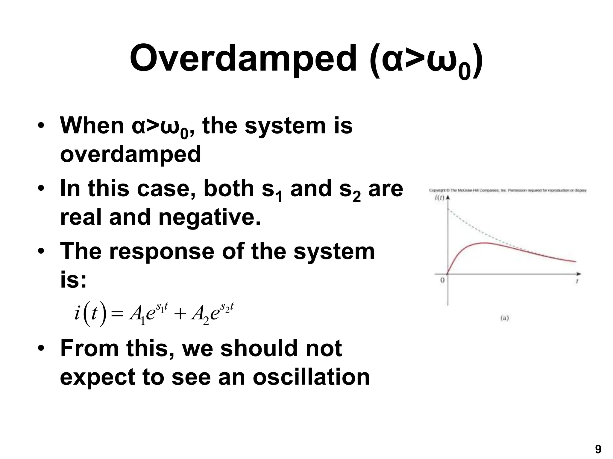
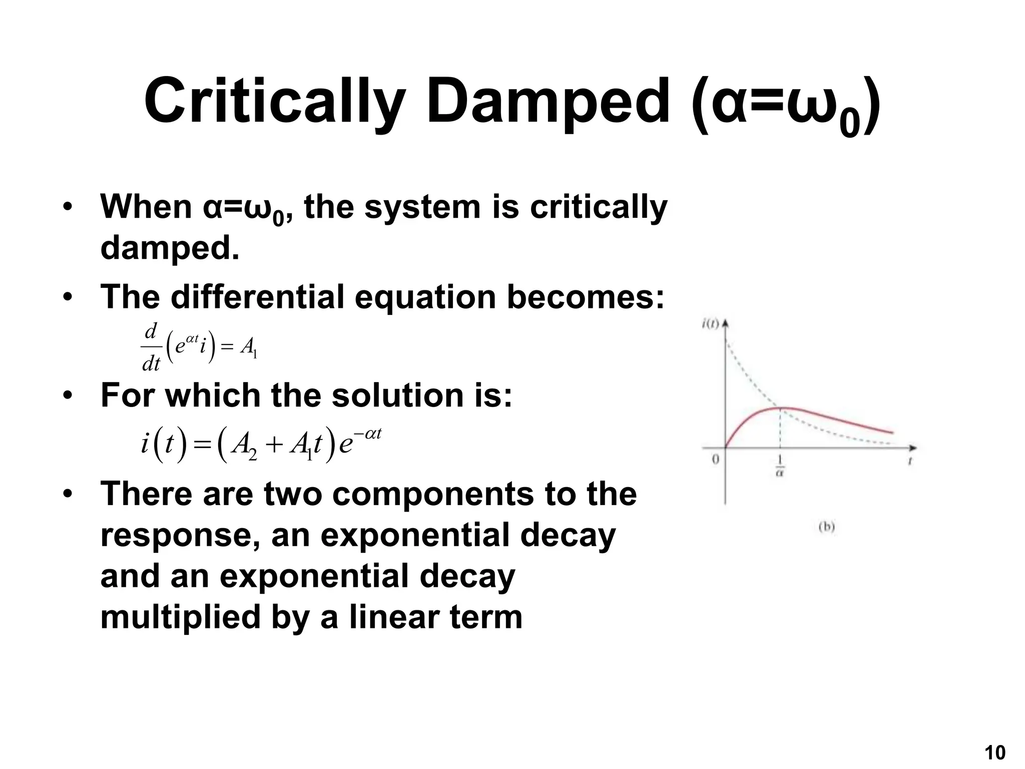
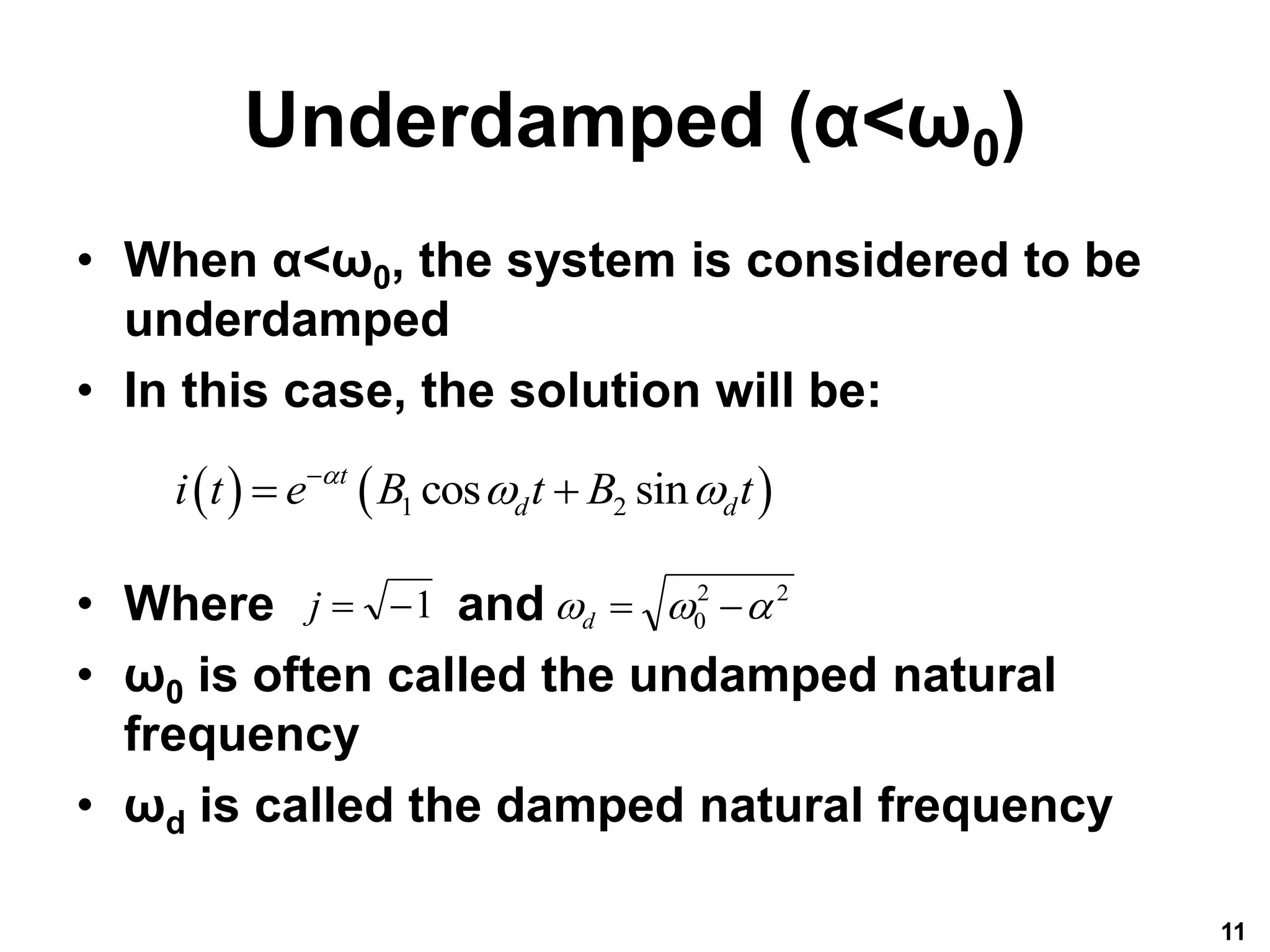
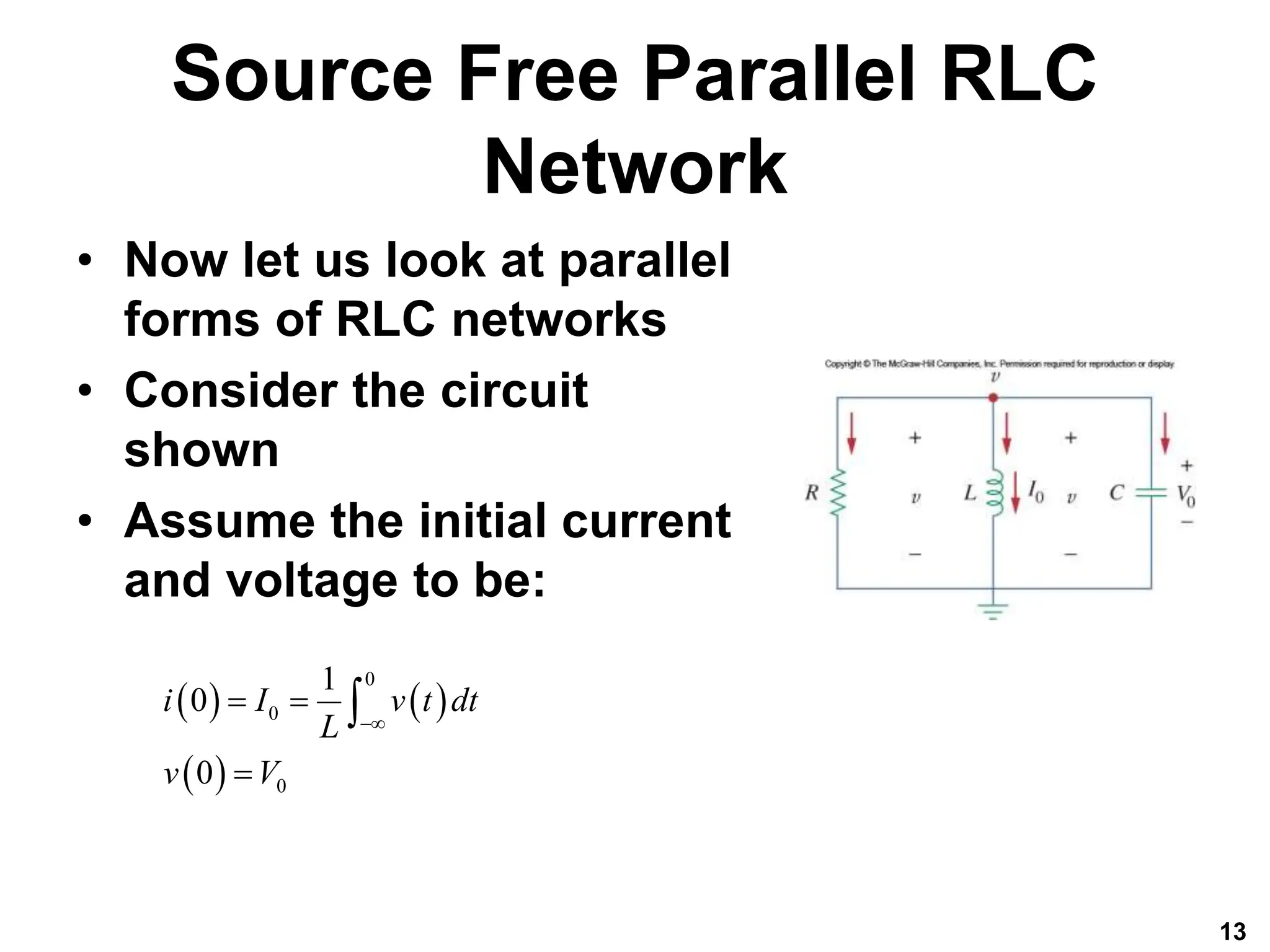
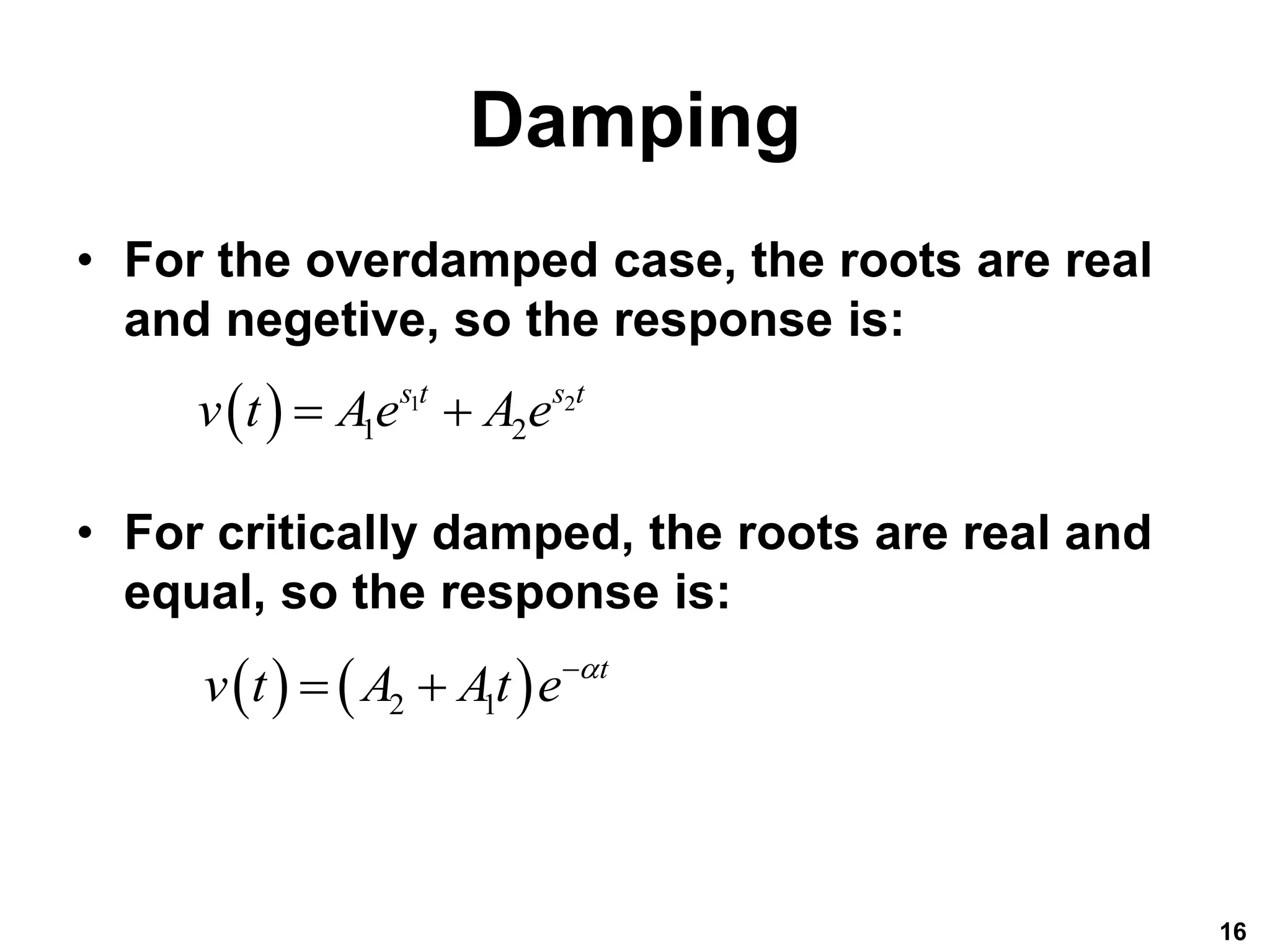
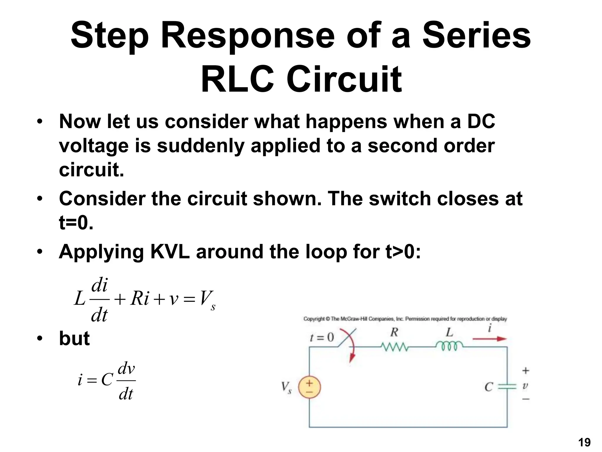
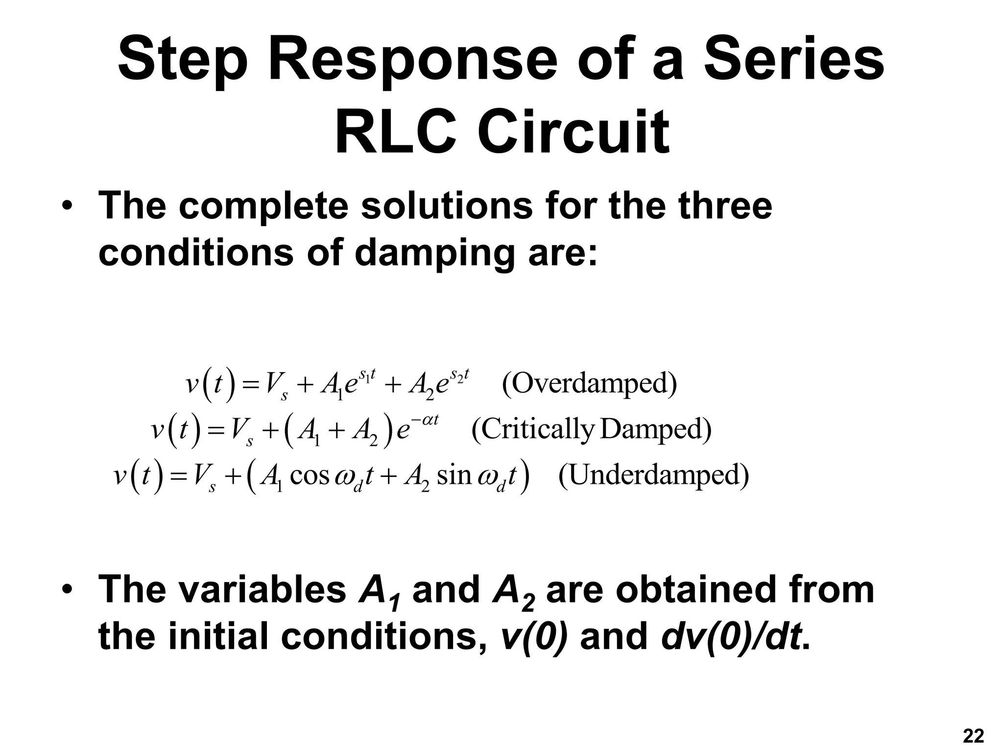
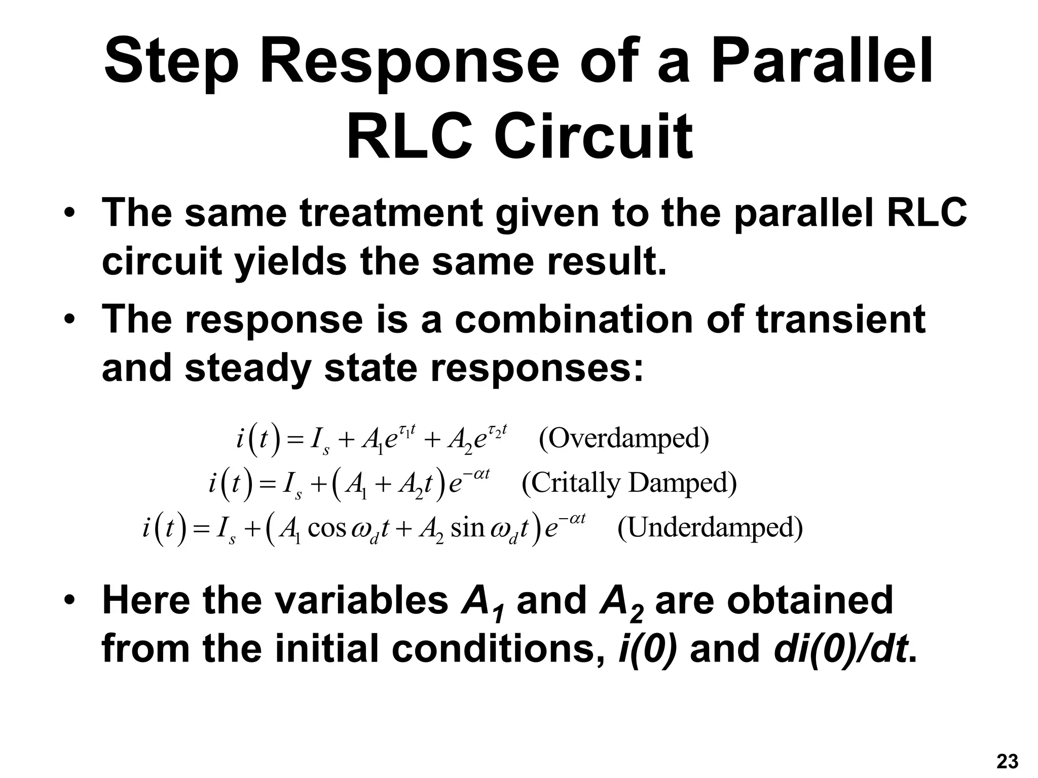
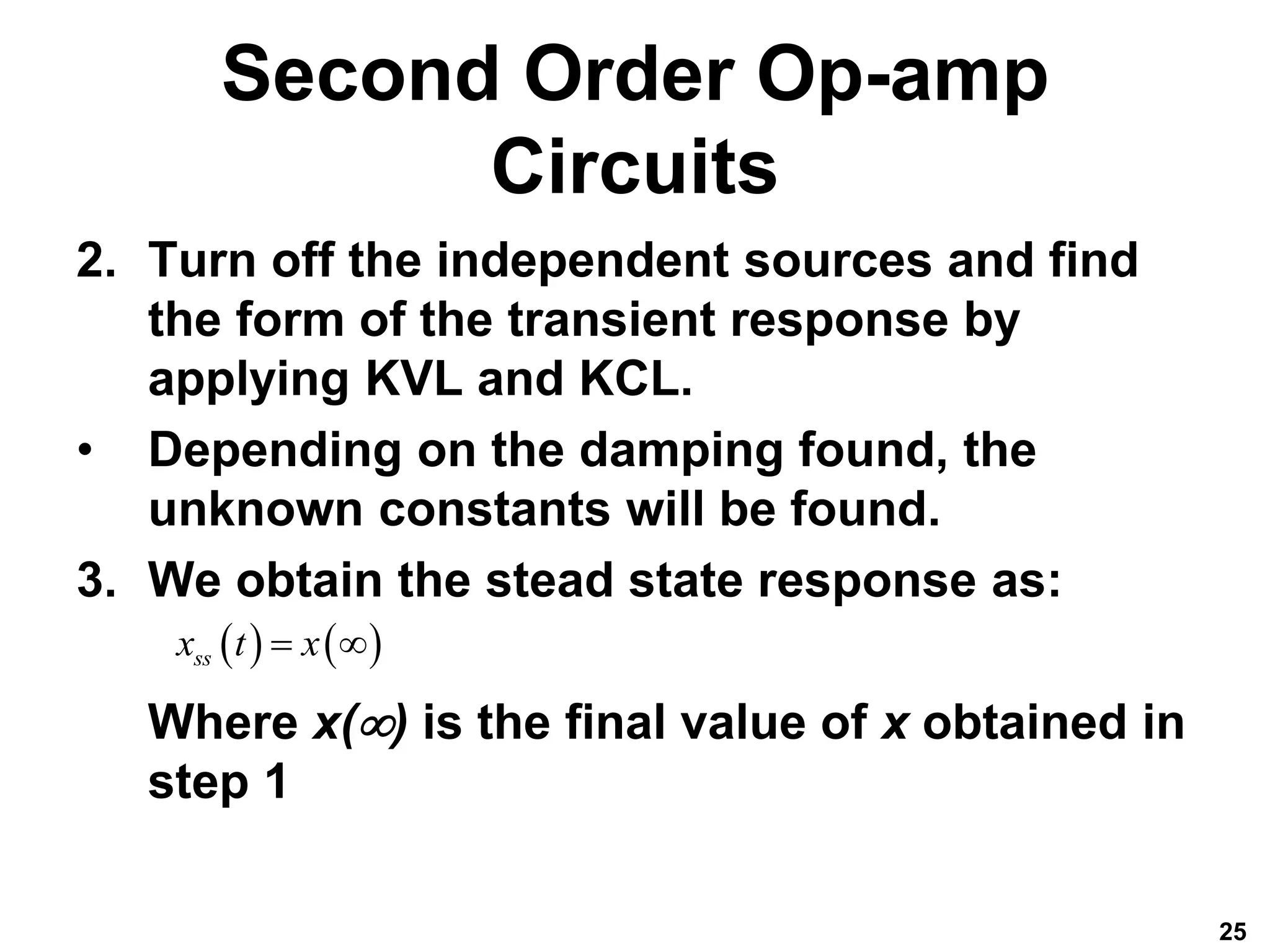
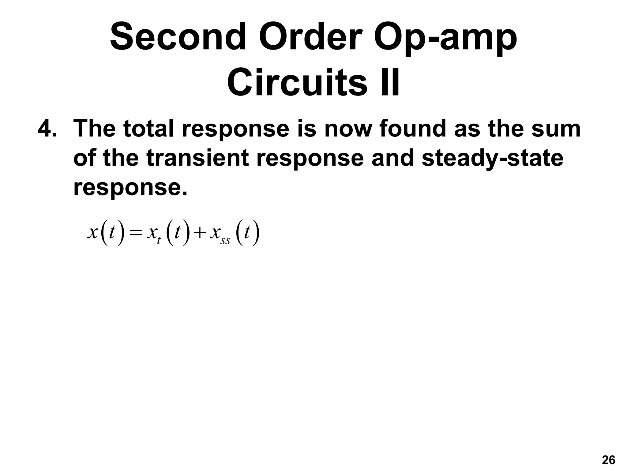
This chapter discusses second order circuits that require second order differential equations to analyze. It covers RLC series and parallel circuits, their step responses, and the concept of duality. Key points: 1) RLC series and parallel circuits form second order systems that have transient responses that can be overdamped, critically damped, or underdamped depending on circuit parameters. 2) The step response of RLC circuits has both a transient and steady-state component. The transient response depends on the damping ratio while the steady-state equals the source voltage/current. 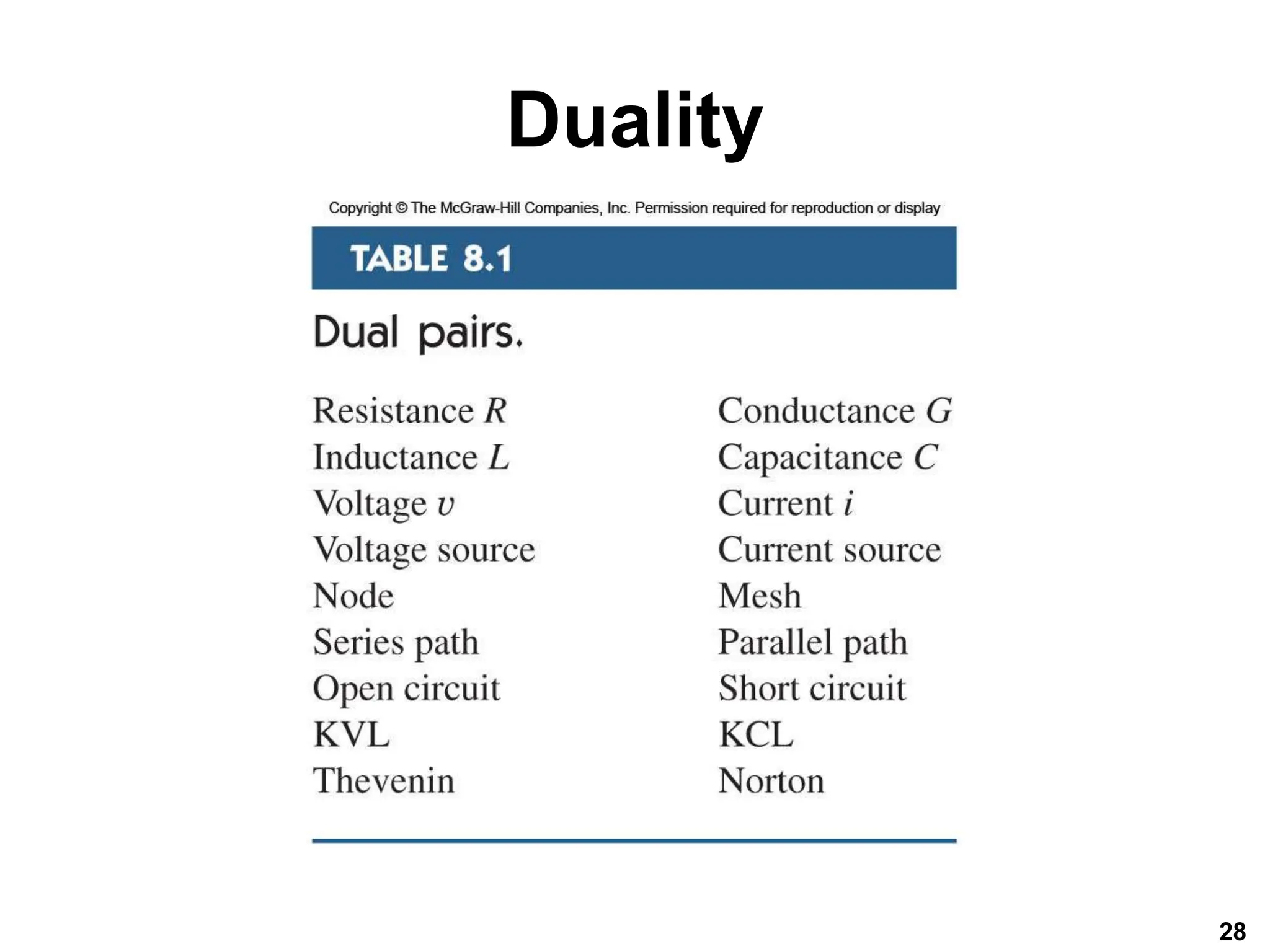3) Duality allows circuits to be related by interchanging complementary elements like resistors and inductors, voltages and currents. It provides a

1. Fundamentals of
Electric Circuits
Chapter 8
Copyright © The McGraw-Hill Companies, Inc. Permission required for reproduction or display.

2. Overview
• The previous chapter introduced the concept of first
order circuits.
• This chapter will expand on that with second order
circuits: those that need a second order differential
equation.
• RLC series and parallel circuits will be discussed in
this context.
• The step response of these circuits will be covered
as well.
• Finally the concept of duality will be discussed.
2

3. Second Order Circuits
• The previous chapter considered
circuits which only required first
order differential equations to
solve.
• However, when more than one
“storage element”, i.e. capacitor
or inductor is present, the
equations require second order
differential equations
• The analysis is similar to what
was done with first order circuits
• This time, though we will only
consider DC independent sources
3

4. Finding Initial and Final
Values
• Working on second order system is harder
than first order in terms of finding initial and
final conditions.
• You need to know the derivatives, dv/dt and
di/dt as well.
• Getting the polarity across a capacitor and
the direction of current through an inductor
is critical.
• Capacitor voltage and inductor current are
always continuous.
4

5. Source Free Series RLC
• Consider the circuit
shown.
• The energy at t=0 is
stored in the capacitor,
represented by V0 and in
the inductor,
represented by I0.
5
 
 
0
0
0
1
0
0
v idt V
C
i I

 



6. Source Free Series RLC
• Applying KVL around the loop:
• The integral can be eliminated by
differentiation:
• Here you can see the second order equation
that results
6
 
1
0
t
di
Ri L i d
dt C
 

  

2
2
0
d i R di i
dt L dt LC
  

7. Source Free Series RLC
• Two initial conditions are needed for solving
this problem.
• The initial current is given.
• The first derivative of the current can also be
had:
• Or
7
 
 
0
0
0 0
di
Ri L V
dt
  
 
 
0 0
0 1
di
RI V
dt L
  

8. Source Free Series RLC
• Based on the first order solutions, we can
expect that the solution will be in exponential
form.
• The equation will then be:
• For which the solutions are:
8
2 1
0
st R
Ae s s
L LC
 
  
 
 
2 2 2 2
1 2
o o
s s
     
       
0
1
2
R
L LC
 
 

9. Overdamped (α>ω0)
• When α>ω0, the system is
overdamped
• In this case, both s1 and s2 are
real and negative.
• The response of the system
is:
• From this, we should not
expect to see an oscillation
9
  1 2
1 2
s t s t
i t Ae A e
 

10. Critically Damped (α=ω0)
• When α=ω0, the system is critically
damped.
• The differential equation becomes:
• For which the solution is:
• There are two components to the
response, an exponential decay
and an exponential decay
multiplied by a linear term
10
  1
t
d
e i A
dt


   
2 1
t
i t A At e 

 

11. Underdamped (α<ω0)
• When α<ω0, the system is considered to be
underdamped
• In this case, the solution will be:
• Where and
• ω0 is often called the undamped natural
frequency
• ωd is called the damped natural frequency
11
1


j 2
2
0 

 

d
   
1 2
cos sin
t
d d
i t e B t B t

 

 

12. Damping and RLC networks
• RLC networks can be charaterized by the
following:
1.The behavior of these networks is captured
by the idea of damping
2.Oscillatory response is possible due to the
presence of two types of energy storage
elements.
3.It is typically difficult to tell the difference
between damped and critically damped
responses.
12

13. Source Free Parallel RLC
Network
• Now let us look at parallel
forms of RLC networks
• Consider the circuit
shown
• Assume the initial current
and voltage to be:
13
   
 
0
0
0
1
0
0
i I v t dt
L
v V

 



14. Source Free Parallel RLC
Network
• Applying KCL to the top node we get:
• Taking the derivative with respect to t gives:
• The characteristic equation for this is:
14
 
1
0
t
v dv
v d C
R L dt
 

  

2
2
1 1
0
d v dv
v
dt RC dt LC
  
2 1 1
0
s s
RC LC
  

15. Source Free Parallel RLC
Network
• From this, we can find the roots of the
characteristic equation to be:
• As in last time, there are three scenarios to
consider.
15
2 2
1,2 0
0
1 1
2
s
RC LC
  
 
   
 

16. Damping
• For the overdamped case, the roots are real
and negetive, so the response is:
• For critically damped, the roots are real and
equal, so the response is:
16
  1 2
1 2
s t s t
v t Ae A e
 
   
2 1
t
v t A At e 

 

17. Underdamped
• In the underdamped case, the roots are
complex and so the response will be:
• To get the values for the constants, we need
to know v(0) and dv(0)/dt.
• To find the second term, we use:
17
   
1 2
cos sin
t
d d
v t e A t A t

 

 
 
0
0
0
0
dv
V
I C
R dt
  

18. Underdamped
• The voltage waveforms will be similar to
those shown for the series network.
• Note that in the series network, we first
found the inductor current and then solved
for the rest from that.
• Here we start with the capacitor voltage and
similarly, solve for the other variables from
that.
18

19. Step Response of a Series
RLC Circuit
• Now let us consider what happens when a DC
voltage is suddenly applied to a second order
circuit.
• Consider the circuit shown. The switch closes at
t=0.
• Applying KVL around the loop for t>0:
• but
19
s
di
L Ri v V
dt
  
dv
i C
dt


20. Step Response of a Series
RLC Circuit
• Substituting for i gives:
• This is similar to the response for the source
free version of the series circuit, except the
variable is different.
• The solution to this equation is a
combination of transient response and
steady state
20
2
2
s
V
d v R dv v
dt L dt LC LC
  
     
t ss
v t v t v t
 

21. Step Response of a Series
RLC Circuit
• The transient response is in the same form
as the solutions for the source free version.
• The steady state response is the final value
of v(t). In this case, the capacitor voltage will
equal the source voltage.
21

22. Step Response of a Series
RLC Circuit
• The complete solutions for the three
conditions of damping are:
• The variables A1 and A2 are obtained from
the initial conditions, v(0) and dv(0)/dt.
22
 
   
   
1 2
1 2
1 2
1 2
(Overdamped)
(CriticallyDamped)
cos sin (Underdamped)
s t s t
s
t
s
s d d
v t V Ae A e
v t V A A e
v t V A t A t

 

  
  
  

23. Step Response of a Parallel
RLC Circuit
• The same treatment given to the parallel RLC
circuit yields the same result.
• The response is a combination of transient
and steady state responses:
• Here the variables A1 and A2 are obtained
from the initial conditions, i(0) and di(0)/dt.
23
 
   
   
1 2
1 2
1 2
1 2
(Overdamped)
(Critally Damped)
cos sin (Underdamped)
t t
s
t
s
t
s d d
i t I Ae A e
i t I A A t e
i t I A t A t e
 


 


  
  
  

24. General Second Order
Circuits
• The principles of the approach to solving the
series and parallel forms of RLC circuits can
be applied to second order circuits in
general:
• The following four steps need to be taken:
1.First determine the initial conditions, x(0) and
dx(0)/dt.
24

25. Second Order Op-amp
Circuits
2. Turn off the independent sources and find
the form of the transient response by
applying KVL and KCL.
• Depending on the damping found, the
unknown constants will be found.
3. We obtain the stead state response as:
Where x() is the final value of x obtained in
step 1
25
   
ss
x t x
 

26. Second Order Op-amp
Circuits II
4. The total response is now found as the sum
of the transient response and steady-state
response.
26
     
t ss
x t x t x t
 

27. Duality
• The concept of duality is a time saving
measure for solving circuit problems.
• It is based on the idea that circuits that
appear to be different may be related to each
other.
• They may use the same equations, but the
roles of certain complimentary elements are
interchanged.
• The following is a table of dual pairs
27

28. Duality
28

29. Duality
• Once you know the solution to one circuit,
you have the solution to the dual circuit.
• Finding the dual of a circuit can be done with
a graphical method:
1.Place a node at the center of each mesh of a
given circuit. Place the reference node
outside the given circuit.
2.Draw lines between the nodes such that each
line crosses an element. Replace the element
with its dual
29

30. Duality
3. To determine the polarity of voltage sources
and of current sources, follow this rule: A
voltage source that produces a positive
(clockwise) mesh current has as its dual a
current source whose reference direction is
from the ground to the nonreference node.
• When in doubt, one can refer to the mesh or
nodal equations of the dual circuit.
30