Spring 2016 Intern at Treasure Data

2016 Spring Intern
@ Treasure Data
2016/4/3 - 2016/6/17
Part 1: Field-Aware Factorization Machines
Part 2: Kernelized Passive-Aggressive
Part 3: ChangeFinder

whoami
Sotaro Sugimoto (杉本宗太郎)
• U. Tokyo B.S. Physics (2016)
• Georgia Tech M.S. Computational Science & Engineering (2016-2018)
• https://github.com/L3Sota
Facebook (Look for the dog)

What will this talk be about?
• Model-based Predictors
• “Reading the future”
• Estimating the value of an important variable
• Determining whether or not some action will occur
• Statistical Anomaly Detection
• The computer monitors a resource and tells us when “something unnatural”
happens

Part 1: Field-Aware Factorization Machines
• What we want to achieve
• SVM to FFM and everything in between
• What’s a Field?
• Pros and Cons

FFM: what we want to achieve
• Prediction: Data goes in, predictions come out
• CTR
• Shopping recommendations
𝑦 = 𝜙(𝒙)
• Regression & Classification
• Regression: Results are real-valued (𝑦, 𝑦 ∈ ℝ)
• Classification: Results are binary (𝑦, 𝑦 ∈ {0,1} and 𝑦, 𝑦 ∈ {±1} are common)
Prediction result
Prediction function
Input vector

Click-Through Rate (CTR) Prediction
• Will user X click my ad? What percentage of users will click my ad? ->
Find the probability that a target of an ad will click through.
Input:
• User ID
• Past ads clicked
• Past conversions made
• Mouse movements
• Favorite websites
Output:
• Whether or not a click-through will occur by user X during a particular session
• Classification

Shopping Recommendations
• Will user X buy this product? What products would this user like to see
next? -> Predict the rating that the user would give to unseen items.
Input:
• User ID
• Past items looked at
• Past items bought
• Past items rated
• Mouse movements
• Favorite product categories
Output:
• Expected ratings for each item (i.e. a list of recommended items when ordered by
rating from highest to lowest)
• Regression
• This is not to say that you can’t make a similar classification problem

So that this…
What is this???
I AM NOT A
FATHER
No thanks…

Becomes this!
Gifts for my girlfriend
Very important.
VERY. Important.
Dead trees! FABULOUS!

FM’s Roots
• FM is a generalized model.
The point of FM was to combine Linear Classification…
• Support Vector Machines (SVM)
…with Matrix-based Approaches.
• Single Value Decomposition (SVD)
• Matrix Factorization (MF)

Support Vector Machines
• Classification
1. Find a plane splitting category 1 from category 2 (H2, H3)
2. Maximize the distance from both categories (H3)
3. New data can be classified with this plane
Image from Wikipedia: https://commons.wikimedia.org/wiki/File:Svm_separating_hyperplanes_(SVG).svg

Support Vector Machines
• Calculation specifics
• Plane is denoted by a vector 𝒘 (the normal vector)
• The prediction function is given by 𝜙 𝑥 = 𝒘, 𝒙 − 𝑏 .
• , is the inner product.
• When using a kernel, the function becomes 𝜙 𝑥 = 𝑖 𝛼𝑖 𝐾 𝒙, 𝒙𝑖 − 𝑏
• e.g. d-dimensional Polynomial Kernel: 𝜙 𝑥 = 𝑖 𝛼𝑖( 𝒙, 𝒙𝑖 + 1) 𝑑
−𝑏
• New data can be classified with 𝑠𝑔𝑛 𝒘, 𝒙 − 𝑏 ∈ {−1, +1}
Image originally from Wikipedia, modified: https://commons.wikimedia.org/wiki/File:Normal_vectors2.svg

FFM’s Roots
• FM is a generalized model.
The point of FM was to combine Linear Classification…
• Support Vector Machines (SVM)
…with Matrix-based Approaches.
• Single Value Decomposition (SVD)
• Matrix Factorization (MF)

Matrix-based
approaches
The difference between SVD and MF (besides the diagonal matrix S) is that MF ignores zero entries in the matrix during factorization, which tends to improve performance.
Image from Qiita: http://qiita.com/wwacky/items/b402a1f3770bee2dd13c

Model Interaction Order Model Equation
Linear Model 1
𝜙1 𝒙 = 𝑤0 +
𝑖=1
𝑛
𝑤𝑖 𝑥𝑖
Poly2 Model 2
𝜙2 𝒙 = 𝜙1 𝑥 +
𝑖<𝑗
𝑛
𝑤𝑖,𝑗 𝑥𝑖 𝑥𝑗
SVM 1 𝜙 𝑆𝑉𝑀 𝒙 = 𝒘, 𝒙 − 𝑏 = 𝜙1(𝒙)
Kernelized SVM n
𝜙 𝐾−𝑆𝑉𝑀 𝒙 =
𝑖=1
𝑛
𝛼𝑖 𝐾 𝒙, 𝒙𝑖 − 𝑏
SVD 2
𝜙 𝑆𝑉𝐷 𝒙 = 𝜙1 𝒙 +
𝑖<𝑗
𝑛
𝑝1,𝑝2
𝑈𝑖,𝑝1
𝑆 𝑝1,𝑝2
𝐼 𝑝2,𝑗 𝑥𝑖 𝑥𝑗
MF 2
𝜙 𝑀𝐹 𝒙 = 𝜙1 𝒙 +
𝑖<𝑗
𝑛
𝑝
𝑈𝑖,𝑝 𝐼 𝑝,𝑗 𝑥𝑖 𝑥𝑗
FM n 𝜙 𝐹𝑀 𝒙 = 𝜙1 𝒙 +
𝑖<𝑗
𝒗𝑖, 𝒗𝑗 𝑥𝑖 𝑥𝑗
FFM 2 (n) 𝜙 𝐹𝐹𝑀 𝒙 = 𝜙1 𝒙 +
𝑖<𝑗
𝒗𝑖,𝛽, 𝒗𝑗,𝛼 𝑥𝑖 𝑥𝑗
Global Bias Single Item Weight
Pairwise

Factorization Machines
• No easy geometric representation 
• The prediction function is given by
𝜙 𝑥 = 𝑤0 + 𝑖=1
𝑛
𝑤𝑖 𝑥𝑖 + 𝑖=1
𝑛
𝑗=𝑖+1
𝑛
𝒗𝑖, 𝒗𝑗 𝑥𝑖 𝑥𝑗 .
• Interactions between components are implicitly modeled with
factorized vectors
• For each 𝒙𝑖, define a vector 𝒗𝑖 with 𝐹 < 𝑛 dimensions.
• 𝒗𝑖, 𝒗𝑗 is used instead of 𝑤𝑖,𝑗. Recall Poly2 is 𝜙2 𝒙 = 𝜙1 𝑥 + 𝑖<𝑗
𝑛
𝑤𝑖,𝑗 𝑥𝑖 𝑥𝑗.
• But wait…
• This is 𝑂(𝐹𝑛2)

Math!
𝑖=1
𝑛
𝑗=𝑖+1
𝑛
𝒗𝑖, 𝒗𝑗 𝑥𝑖 𝑥𝑗 =
𝑗=1
𝑛
𝑖=𝑗+1
𝑛
=
1
2 𝑖=1
𝑛
𝑗=1
𝑛
𝒗𝑖, 𝒗𝑗 𝑥𝑖 𝑥𝑗 −
𝑖=1
𝑛
𝒗𝑖, 𝒗𝑖 𝑥𝑖 𝑥𝑖
=
1
2 𝑘=1
𝐹
𝑖=1
𝑛
𝑗=1
𝑛
𝑣𝑖,𝑘 𝑣𝑗,𝑘 𝑥𝑖 𝑥𝑗 −
𝑖=1
𝑛
𝒗𝑖
2 𝑥𝑖
2
=
1
2 𝑘=1
𝐹
𝑖=1
𝑛
𝑣𝑖,𝑘 𝑥𝑖
𝑗=1
𝑛
𝑣𝑗,𝑘 𝑥𝑗 −
𝑖=1
𝑛
𝒗𝑖
2 𝑥𝑖
2
=
1
2 𝑘=1
𝐹
𝑖=1
𝑛
𝑥𝑖 𝑣𝑖,𝑘
2
−
𝑖=1
𝑛
𝑣𝑖,𝑘
2
𝑥𝑖
2
𝒗𝑖, 𝒗𝑗 𝑥𝑖 𝑥𝑗= 𝒗𝑗, 𝒗𝑖 𝑥𝑗 𝑥𝑖
1,1 1,2 1,3 1,4 1,5
2,1 2,2 2,3 2,4 2,5
3,1 3,2 3,3 3,4 3,5
4,1 4,2 4,3 4,4 4,5
5,1 5,2 5,3 5,4 5,5
𝑖=1
2
𝑗=1
2
𝑎𝑖 𝑏𝑗
=𝑎1 𝑏1 + 𝑎1 𝑏2 + 𝑎2 𝑏1 + 𝑎2 𝑏2
= (𝑎1 + 𝑎2)(𝑏1 + 𝑏2)
𝑗
𝑖

Factorization Machines
Substitute in the previous calculations:
𝜙 𝑥 = 𝑤0 +
𝑖=1
𝑛
𝑤𝑖 𝑥𝑖 +
1
2 𝑘=1
𝐹
𝑖=1
𝑛
𝑣𝑖,𝑘 𝑥𝑖
2
−
𝑖=1
𝑛
𝑣𝑖,𝑘
2
𝑥𝑖
2
Works wonders on sparse data!
• Factorization allows implicit interaction modeling, i.e. we can infer interaction
strengths from similar data
• Factorization vectors only depend on one data point so calculations are 𝑂(𝐹𝑛).
• In fact, with a sparse representation the complexity is 𝑶(𝑭𝒎), where 𝑚 is the average
number of non-zero components.
But wait…
• Not as useful for dense data (use SVM for dense data classifications)
𝑂(1) 𝑂(𝑛) 𝑂 𝐹𝑛
𝜙 𝑥 = 𝑤0 +
𝑖=1
𝑛
𝑤𝑖 𝑥𝑖 +
𝑖=1
𝑛
𝑗=𝑖+1
𝑛

Field-Aware Factorization Machines
• A more powerful FM
• The prediction function is given by
𝜙 𝑥 = 𝑤0 + 𝑖=1
𝑛
𝑤𝑖 𝑥𝑖 + 𝑖<𝑗
𝑛
𝒗𝑖,𝛽, 𝒗𝑗,𝛼 𝑥𝑖 𝑥𝑗 .
• Wait, what changed?
• There is an additional subscript on 𝒗, known as the field.
• Note: The constant and linear terms remain the same.

Field-Aware Factorization Machines
These are
fields
These are
features

Field-Aware Factorization Machines (cont.)
𝜙 𝑥 = 𝑤0 +
𝑖=1
𝑛
𝑤𝑖 𝑥𝑖 +
𝑖<𝑗
𝑛
• We specify a 𝒗 based on the current feature 𝑖 of the input vector 𝒙
and the field 𝛽 of the other feature 𝑗.
• In other words, for each pair of features (𝑖, 𝑗) we can specify two
vectors 𝒗, one where we use the field 𝛼 of 𝑖 (i.e. 𝒗𝑗,𝛼), and another
where we use the field 𝛽 of 𝑗 (i.e. 𝒗𝑖,𝛽).

Worked Example: 1 Data Point
• Sotaro went to see Zootopia!
• I haven’t actually seen Zootopia yet.
• Let’s guess what his rating will be. -> Regression
Field Abbrev. Feature Abbrev. Value
Users u L3Sota s 1
Movies m Zootopia z 1
Genre g Comedy c 1
Genre g Drama d 1
Price pp Price p 1200

Linear Model
Users u L3Sota s 1
Genre g Comedy c 1
Genre g Drama d 1
𝜙1 𝒙 = 𝑤0 + 𝑤𝑠 𝑥 𝑠 + 𝑤𝑧 𝑥 𝑧 + 𝑤𝑐 𝑥 𝑐 + 𝑤 𝑑 𝑥 𝑑 + 𝑤 𝑝 𝑥 𝑝
= 1𝑤𝑠 + 1𝑤𝑧 + 1𝑤𝑐 + 1𝑤 𝑑 + 1200𝑤 𝑝
• A single vector is sufficient to hold all the weights.

Poly2 Model
Users u L3Sota s 1
Genre g Comedy c 1
Genre g Drama d 1
𝜙2 𝒙 = 𝑤0 + 𝑤𝑠 𝑥 𝑠 + 𝑤𝑧 𝑥 𝑧 + 𝑤𝑐 𝑥 𝑐 + 𝑤 𝑑 𝑥 𝑑 + 𝑤 𝑝 𝑥 𝑝
+𝒘 𝒔,𝒛 𝒙 𝒔 𝒙 𝒛 + 𝒘 𝒔,𝒄 𝒙 𝒔 𝒙 𝒄 + 𝒘 𝒔,𝒅 𝒙 𝒔 𝒙 𝒅 + 𝒘 𝒔,𝒑 𝒙 𝒔 𝒙 𝒑
+𝒘 𝒛,𝒄 𝒙 𝒛 𝒙 𝒄 + 𝒘 𝒛,𝒅 𝒙 𝒛 𝒙 𝒅 + 𝒘 𝒛,𝒑 𝒙 𝒛 𝒙 𝒑
+𝒘 𝒄,𝒅 𝒙 𝒄 𝒙 𝒅 + 𝒘 𝒄,𝒑 𝒙 𝒄 𝒙 𝒑
+𝒘 𝒅,𝒑 𝒙 𝒅 𝒙 𝒑
𝑤0, 𝑤𝑠, 𝑤𝑧, 𝑤𝑐, 𝑤 𝑑, 𝑤 𝑝
𝑤𝑠,𝑧, 𝑤𝑠,𝑐, 𝑤𝑠,𝑑, 𝑤𝑠,𝑝,
𝑤𝑧,𝑐, 𝑤 𝑧,𝑑, 𝑤𝑧,𝑝,
𝑤𝑐,𝑑, 𝑤𝑐,𝑝,
𝑤 𝑑,𝑝

FM Model
Users u L3Sota s 1
Genre g Comedy c 1
Genre g Drama d 1
𝜙 𝐹𝑀 𝒙 = 𝑤0 + 𝑤𝑠 𝑥 𝑠 + 𝑤𝑧 𝑥 𝑧 + 𝑤𝑐 𝑥 𝑐 + 𝑤 𝑑 𝑥 𝑑 + 𝑤 𝑝 𝑥 𝑝
+ 𝒗 𝑠, 𝒗 𝑧 𝑥 𝑠 𝑥 𝑧 + 𝒗 𝑠, 𝒗 𝑐 𝑥 𝑠 𝑥 𝑐 + 𝒗 𝑠, 𝒗 𝑑 𝑥 𝑠 𝑥 𝑑 + 𝒗 𝑠, 𝒗 𝑝 𝑥 𝑠 𝑥 𝑝
+ 𝒗 𝑧, 𝒗 𝑐 𝑥 𝑧 𝑥 𝑐 + 𝒗 𝑧, 𝒗 𝑑 𝑥 𝑧 𝑥 𝑑 + 𝒗 𝑧, 𝒗 𝑝 𝑥 𝑧 𝑥 𝑝
+ 𝒗 𝑐, 𝒗 𝑑 𝑥 𝑐 𝑥 𝑑 + 𝒗 𝑐, 𝒗 𝑝 𝑥 𝑐 𝑥 𝑝
+ 𝒗 𝑑, 𝒗 𝑝 𝑥 𝑑 𝑥 𝑝
𝑤0, 𝑤𝑠, 𝑤𝑧, 𝑤𝑐, 𝑤 𝑑, 𝑤 𝑝
𝒗 𝑠, 𝒗 𝑧, 𝒗 𝑐, 𝒗 𝑑, 𝒗 𝑝

FFM Model
Users u L3Sota s 1
Genre g Comedy c 1
Genre g Drama d 1
𝜙 𝐹𝑀𝑀 𝒙 = 𝑤0 + 𝑤𝑠 𝑥 𝑠 + 𝑤𝑧 𝑥 𝑧 + 𝑤𝑐 𝑥 𝑐 + 𝑤 𝑑 𝑥 𝑑 + 𝑤 𝑝 𝑥 𝑝
+ 𝒗 𝑠, 𝑚 , 𝒗 𝑧, 𝑢 𝑥 𝑠 𝑥 𝑧 + 𝒗 𝑠, 𝑔 , 𝒗 𝑐, 𝑢 𝑥 𝑠 𝑥 𝑐 + 𝒗 𝑠, 𝑔 , 𝒗 𝑑, 𝑢 𝑥 𝑠 𝑥 𝑑 + 𝒗 𝑠, 𝑝𝑝 , 𝒗 𝑝, 𝑢 𝑥 𝑠 𝑥 𝑝
+ 𝒗 𝑧, 𝑔 , 𝒗 𝑐, 𝑚 𝑥 𝑧 𝑥 𝑐 + 𝒗 𝑧, 𝑔 , 𝒗 𝑑, 𝑚 𝑥 𝑧 𝑥 𝑑 + 𝒗 𝑧, 𝑝𝑝 , 𝒗 𝑝, 𝑚 𝑥 𝑧 𝑥 𝑝
+ 𝒗 𝑐, 𝑔 , 𝒗 𝑑, 𝑔 𝑥 𝑐 𝑥 𝑑 + 𝒗 𝑐, 𝑝𝑝 , 𝒗 𝑝, 𝑔 𝑥 𝑐 𝑥 𝑝
+ 𝒗 𝑑, 𝑝𝑝 , 𝒗 𝑝, 𝑔 𝑥 𝑑 𝑥 𝑝 𝑤0, 𝑤𝑠, 𝑤𝑧, 𝑤𝑐, 𝑤 𝑑, 𝑤 𝑝
𝒗 𝑠,𝑚, 𝒗 𝑠,𝑔, 𝒗 𝑠,𝑝𝑝
𝒗 𝑧,𝑢, 𝒗 𝑧,𝑔, 𝒗 𝑧,𝑝𝑝
𝒗 𝑐,𝑢, 𝒗 𝑐,𝑚, 𝒗 𝑐,𝑔, 𝒗 𝑐,𝑝𝑝
𝒗 𝑑,𝑢, 𝒗 𝑑,𝑚, 𝒗 𝑑,𝑔, 𝒗 𝑑,𝑝𝑝
𝒗 𝑝,𝑢, 𝒗 𝑝,𝑚, 𝒗 𝑝,𝑔

Pros and Cons: FFM
• Pros
• Higher prediction accuracy (i.e. the model is more expressive than FM)
• Cons
• 𝑂(𝐹𝑓𝑚) computation complexity (𝑓: number of fields)
𝜙 𝑥 = 𝑤0 + 𝑖=1
𝑛
𝑤𝑖 𝑥𝑖 + 𝑖<𝑗
𝑛
where 𝛽 is the field of 𝑗 and 𝛼 is the field of 𝑖
• Can’t split the inner product into two independent sums! -> Double loop
• FM was 𝑂(𝐹𝑚).
• Data structures need to understand the field of each component (feature) in
the input vector. -> More memory consumption

Status of FFM within Hivemall
• Pull request merged (#284)
• https://github.com/myui/hivemall/pull/284
• Will probably be in next release(?)
• train_ffm(array<string> x, double y[, const string options])
• Trains the internal FFM model using a (sparse) vector x and target y.
• Training uses Stochastic Gradient Descent (SGD).
• ffm_predict(m.model_id, m.model, data.features)
• Calculates a prediction from the given FFM model and data vector.
• The internal FFM model is referenced as ffm_model m

Part 2: Kernelized Passive-Aggressive
• Quite Similar to SVM
• Pros and Cons

KPA: What we want to achieve
• Prediction: Same as FFM
• Regression & Classification: Same as FFM
• Passive-Aggressive uses a linear model -> similar to Support Vector Machines

Quite Similar to SVM
• SVM Model is 𝜙 𝑆𝑉𝑀 𝒙 = 𝒘, 𝒙 − 𝑏
• Passive-Aggressive Model is 𝜙 𝑃𝐴 𝒙 = 𝒘, 𝒙 − 𝑏
• Additionally, PA uses a margin 𝜖, which has different
meanings for classification and regression.
What’s the difference?
• Passive-Aggressive models don’t update
their weights when a new data point is correctly
classified/a new data point is within the
regression range.
• PA is an online algorithm (real-time learning)
• SVM generally uses batch learning
Classification
Regression
Images and equations from slides at http://ttic.uchicago.edu/~shai/ppt/PassiveAggressive.ppt

But That’s Regular Passive-Aggressive
What’s Kernelized PA, then?
• Kernelization means instead of using 𝜙 𝑃𝐴 𝒙 = 𝒘, 𝒙 − 𝑏, we introduce a
kernel function 𝐾 𝒙, 𝒙𝑖 which increases the expressiveness of the
algorithm, i.e. 𝜙 𝐾𝑃𝐴 𝒙 = 𝑖 𝛼𝑖 𝐾 𝒙, 𝒙𝑖 .
• This is geometrically interpreted as mapping each data point into a corresponding
point in a higher dimensional space.
• In our case we used a Polynomial Kernel (of degree 𝑑 with constant 𝑐)
which can be expressed as follows:
𝐾 𝒙, 𝒙𝑖 = 𝒙, 𝒙𝑖 + 𝑐 𝑑
• E.g. when 𝑑 = 2, 𝐾 𝒙, 𝒙𝑖 = 𝒙, 𝒙𝑖
2 + 2𝑐 𝒙, 𝒙𝑖 + 𝑐2
• This gives us a model of higher degree, i.e. a model that has interactions
between features!
• Note: The same methods can be used to make a Kernelized SVM too!

Regression? Model
Order
Categories Model Equation
Linear Model N 1 1
𝜙1 𝒙 = 𝑤0 +
𝑖=1
𝑛
𝑤𝑖 𝑥𝑖
Poly2 Model Y 2 1
𝜙2 𝒙 = 𝜙1 𝑥 +
𝑖<𝑗
𝑛
𝑤𝑖,𝑗 𝑥𝑖 𝑥𝑗
SVM N 1 1 𝜙 𝑆𝑉𝑀 𝒙 = 𝒘, 𝒙 − 𝑏 = 𝜙1(𝒙)
Kernelized SVM N n 1
𝜙 𝐾−𝑆𝑉𝑀 𝒙 =
𝑖=1
𝑛
𝛼𝑖 𝐾 𝒙, 𝒙𝑖 − 𝑏
SVD Y 2 2
𝜙 𝑆𝑉𝐷 𝒙 = 𝜙1 𝒙 +
𝑖<𝑗
𝑛
𝑝1,𝑝2
𝑈𝑖,𝑝1
𝑆 𝑝1,𝑝2
𝐼 𝑝2,𝑗 𝑥𝑖 𝑥𝑗
MF Y 2 2
𝜙 𝑀𝐹 𝒙 = 𝜙1 𝒙 +
𝑖<𝑗
𝑛
𝑝
𝑈𝑖,𝑝 𝐼 𝑝,𝑗 𝑥𝑖 𝑥𝑗
FM Y n n 𝜙 𝐹𝑀 𝒙 = 𝜙1 𝒙 +
𝑖<𝑗
FFM Y 2 (n) n 𝜙 𝐹𝑀 𝒙 = 𝜙1 𝒙 +
𝑖<𝑗
Global Bias Item/User Bias
Pairwise

Pros and Cons: KPA
• Pros
• A higher order model generally means better classification/regression results
• Cons
• A Polynomial Kernel of degree 𝑑 generally has a computational complexity of
𝑂(𝑛 𝑑
)
• However, this can be avoided, especially where input is sparse!

Status of Kernelized Passive-Aggressive in
Hivemall
• KPA for classification is complete
• Also includes modified PA algorithms PA-I and PA-II in kernelized form
• i.e. KPA-I, KPA-II
• No pull request yet
• https://github.com/L3Sota/hivemall/tree/feature/kernelized_pa
• Didn’t get around to writing the pull request
• Code has been reviewed.
• Includes options for faster processing of the kernel, such as Kernel
Expansion and Polynomial Kernel with Inverted Indices (PKI)
• Don’t ask me why it’s not called PKII

Part 3: ChangeFinder
• How ChangeFinder Works
• What ChangeFinder can and can’t do

ChangeFinder: what we want to achieve
• Anomaly/Change-Point Detection: Data goes in, anomalies come out
• What’s the difference? -> Lone outliers are detected as anomalies and
long-lasting/permanent changes in behavior are detected as change-
points.
• Anomalies: Performance statistics (98th percentile response time, CPU usage)
go in; momentary dips in performance (anomalies) may be signs of network
or processing bottlenecks.
• Change-Points: Activity (port 135 traffic, SYN requests, credit card usage) goes
in; explosive increases in activity (change-points) may be signs of an attack
(virus, flood, identity theft).

How ChangeFinder Works
Anomaly Detection:
1. We assume the data follows a pattern and attempt to model it.
2. The current model 𝜃𝑡 gives a probability distribution 𝑝(⋅ | 𝜃𝑡 )for
the next data point, i.e. the probability that 𝑥 𝑡+1 ∈ 𝑎, 𝑏 is
𝑎
𝑏
𝑝( 𝑥 𝑡+1| 𝜃𝑡 )𝑑𝑥.
3. Once the next datum arrives, we can calculate a score from the
probability distribution
𝑆𝑐𝑜𝑟𝑒 𝑥 𝑡+1 = −log(𝑝 𝑥 𝑡+1 𝜃𝑡 )
4. If the score is greater than a preset threshold, an anomaly has been
detected.

Change-Point Detection:
1. We assume the running mean of the anomaly scores
𝑦𝑡 =
1
𝑊 𝑖=1
𝑊
𝑆𝑐𝑜𝑟𝑒(𝑥𝑡−𝑖 )
follows a pattern and attempt to model it.
2. The current model 𝜙 𝑡 gives a probability distribution 𝑝(⋅ | 𝜙 𝑡 )for the next
score, i.e. the probability that 𝑦𝑡+1 ∈ 𝑎, 𝑏 is 𝑎
𝑏
𝑝( 𝑦𝑡+1| 𝜙 𝑡 )𝑑𝑥.
3. Once the next datum arrives, we can calculate a score from the probability
distribution
𝑆𝑐𝑜𝑟𝑒 𝑦𝑡+1 = −log(𝑝 𝑦𝑡+1 𝜙 𝑡 )
4. If the score is greater than a preset threshold, a change-point has been
detected.

1. We assume an 𝑛 -degree Autoregressive model 𝜃𝑡 = 𝝁, 𝐴𝑖, 𝜺 𝑡 :
𝒙 𝑡 = 𝝁 +
𝑖=1
𝑛
𝐴𝑖(𝒙 𝑡−𝑖 − 𝝁) + 𝜺 𝑡
• 𝝁: The average of the model
• 𝐴𝑖: The model matrices, which determine how previous data affects
the next data point
• 𝜺 𝑡: A normally distributed error term following 𝒩(0, Σ)
AR model example graphs obtained from http://paulbourke.net/miscellaneous/ar/

2. Given the parameters of the model, we calculate an estimate for
the next data point:
𝒙 𝑡 = 𝝁 +
𝑖=1
𝑛
𝐴𝑖(𝒙 𝑡−𝑖− 𝝁)
• Hats denote “statistically estimated value”
3. We then receive a new input 𝒙 𝑡, and calculate the estimation error
𝒙 𝑡 − 𝒙 𝑡. Assuming the model parameters are (mostly) correct, this
expression evaluates to 𝜺 𝑡, which we know is distributed according
to 𝒩(0, Σ).

4. We can therefore calculate the score as
𝑆𝑐𝑜𝑟𝑒 𝒙 𝑡 = − log 𝑝 𝒙 𝑡 𝜃𝑡
= −
1
𝑑
log
exp −
1
2
𝒙 𝑡 − 𝜇 𝑇
Σ−1
𝒙 𝑡 − 𝜇
2𝜋 −
𝑑
2( Σ −
1
2)
• Our estimate of the model is never perfect, so we should update the model
parameters each time a new data point comes in!
• We also need to update the model parameters whenever we encounter a change-
point, since the series has completely changed behavior.
5. After calculating the score for 𝒙 𝑡, we assume that 𝒙 𝑡 follows the same
time series and update our model parameter estimates 𝜃𝑡 = 𝝁, 𝐴𝑖, 𝜺 𝑡

What ChangeFinder can and can’t do
• ChangeFinder can detect anomalies and change-points.
• ChangeFinder can adapt to slowly changing data without sending
false positives.
• ChangeFinder can be adjusted to be more/less sensitive.
• Window size, Forgetfulness, Detection Threshold
• ChangeFinder can’t distinguish an infinitely large anomaly from a
change-point.
• ChangeFinder can’t detect small change-points.
• ChangeFinder can’t correctly detect anything at the beginning of the
dataset.

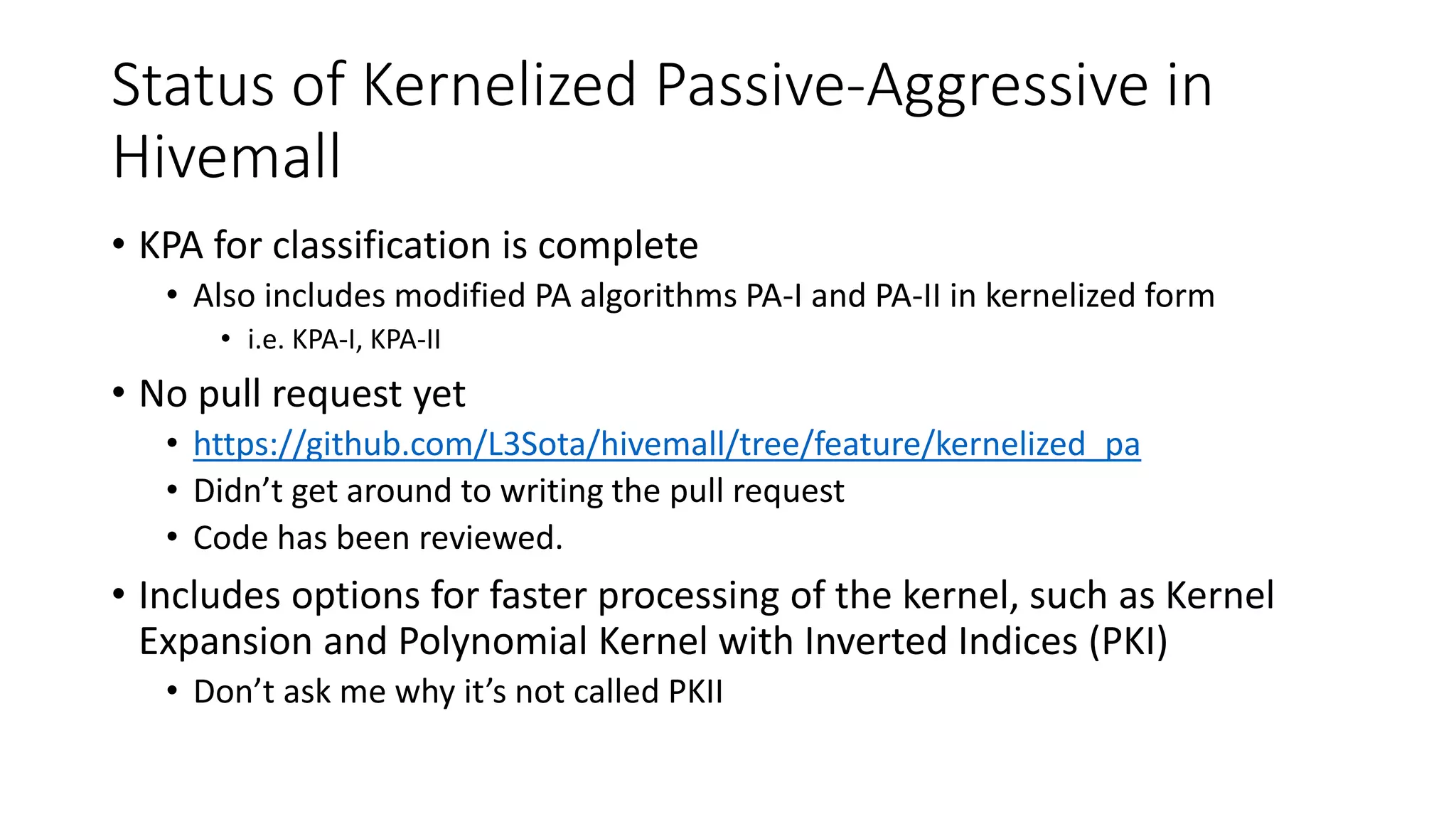
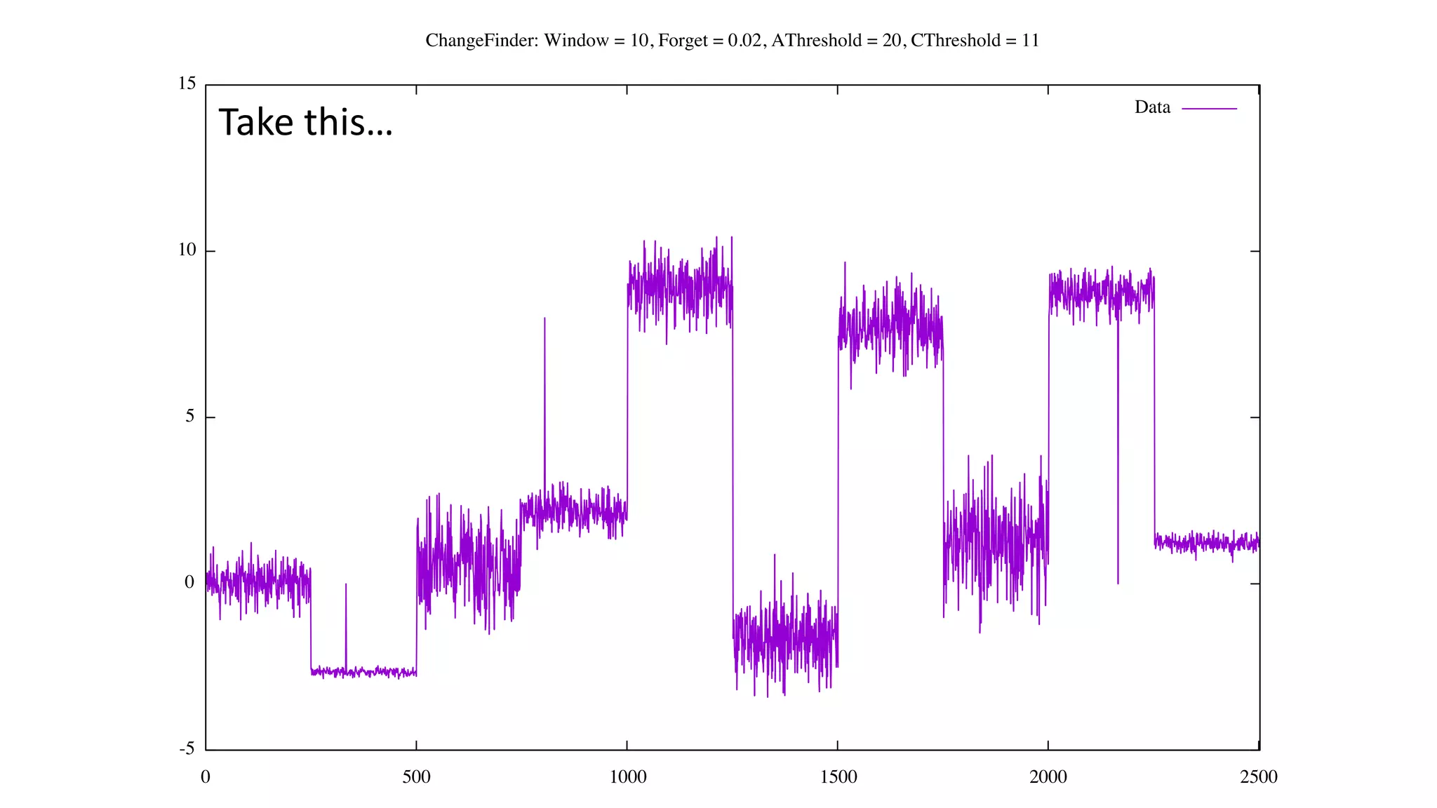
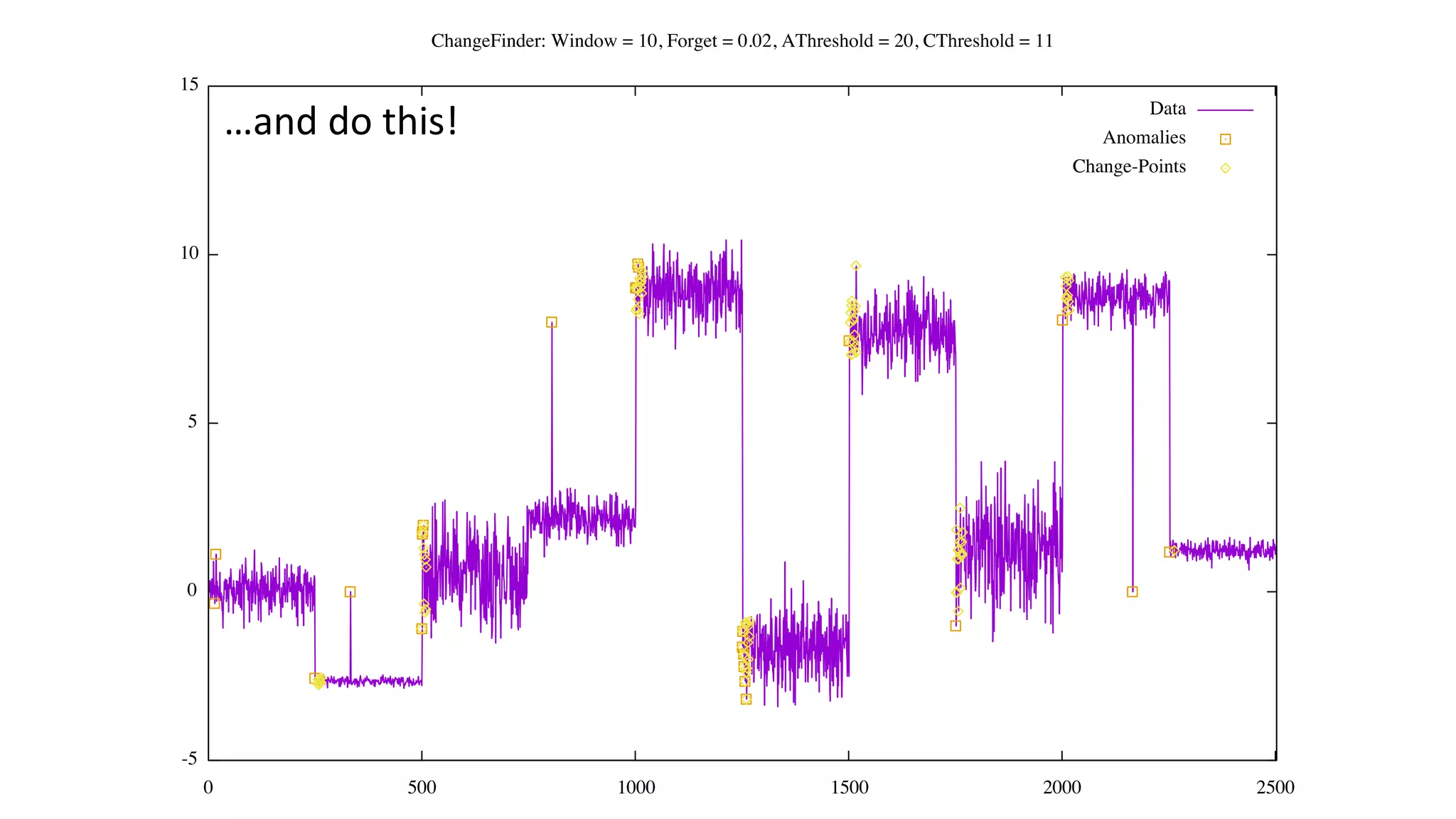
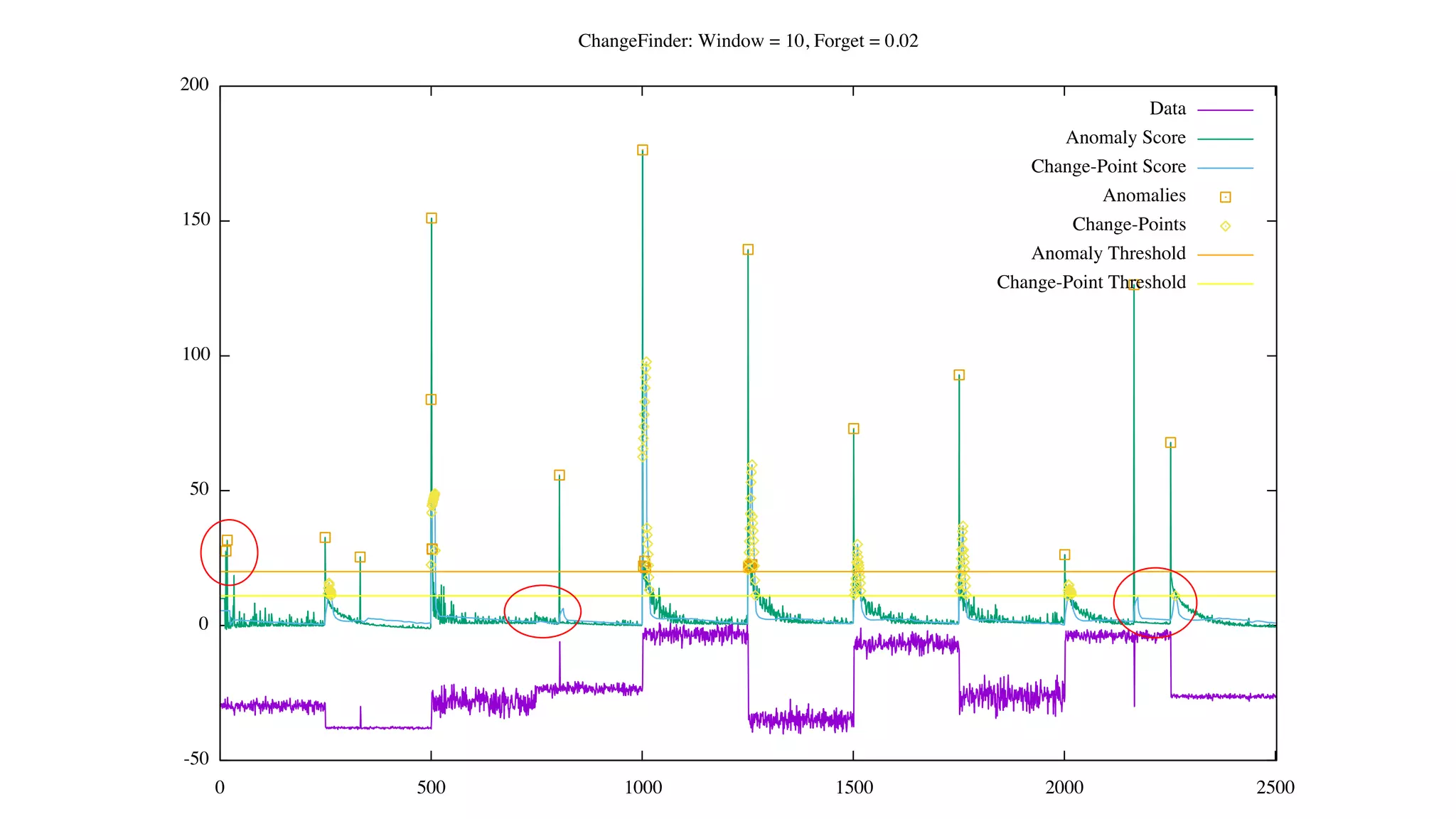
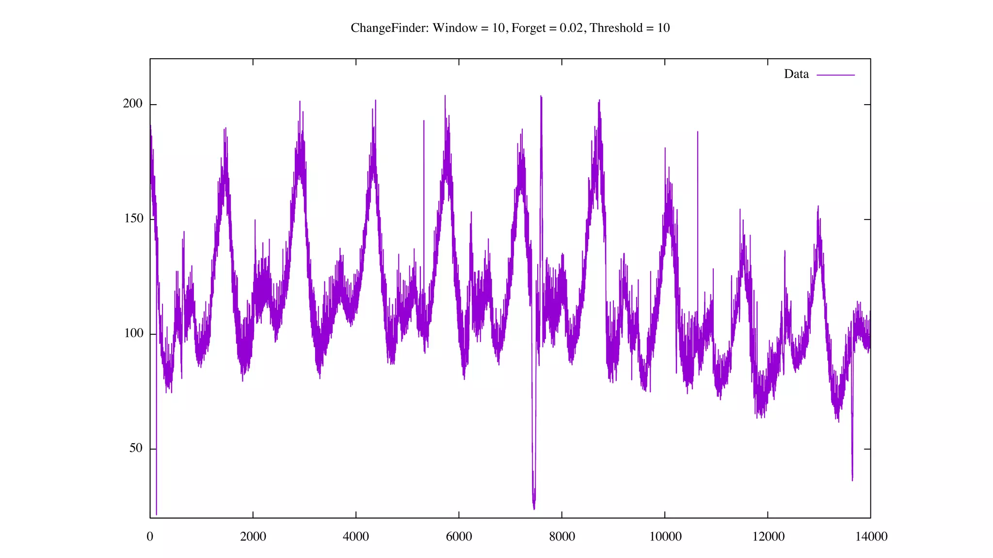
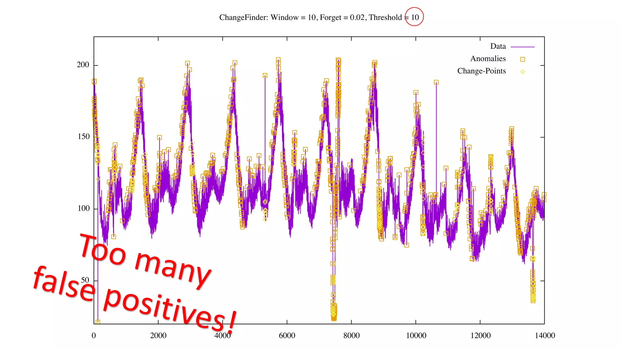
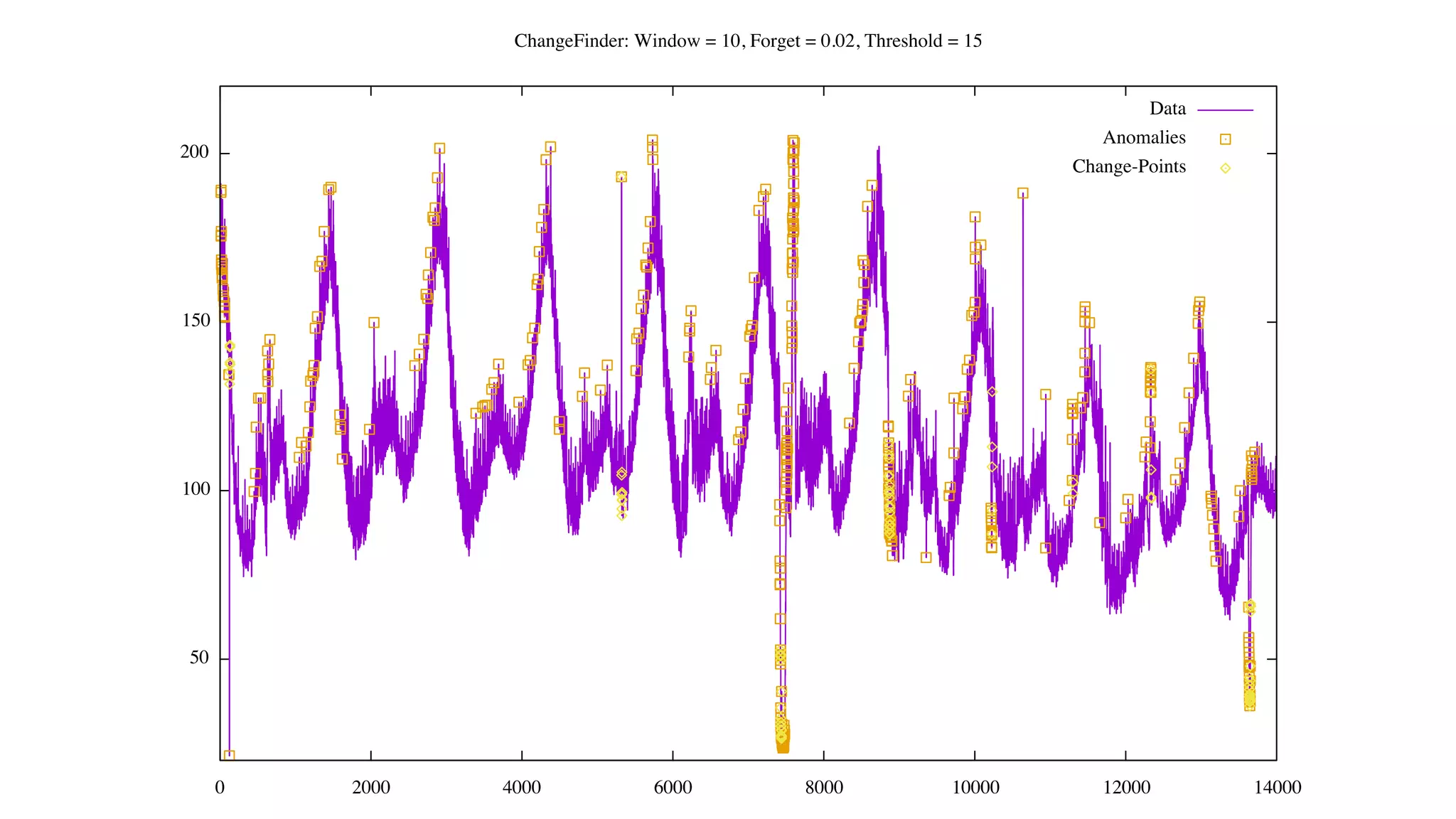
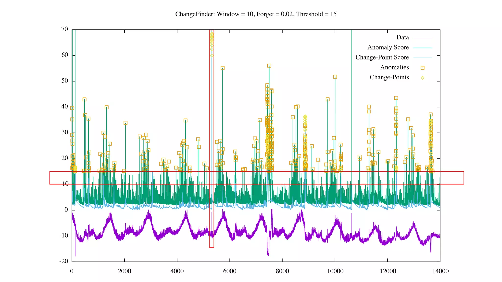
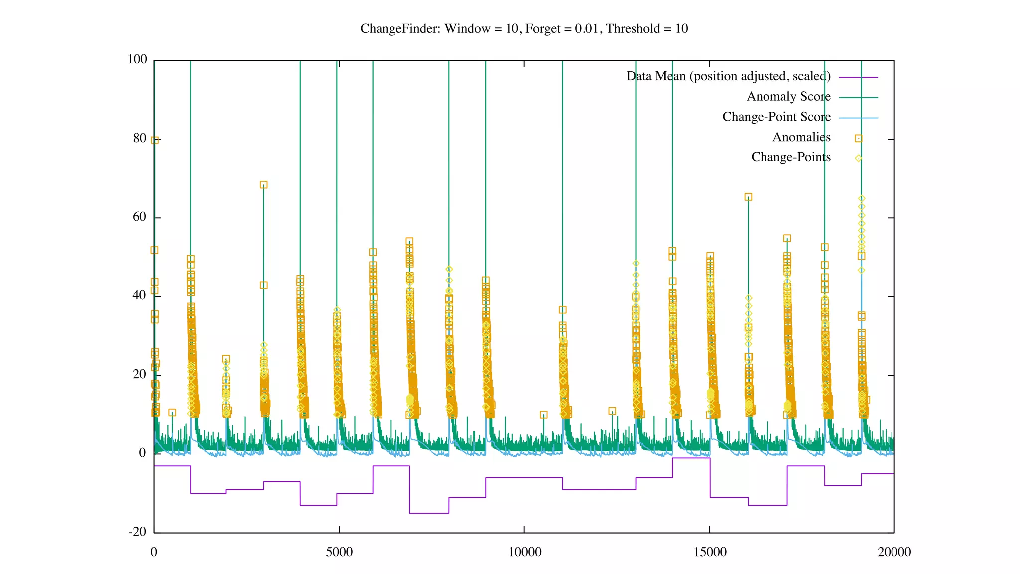
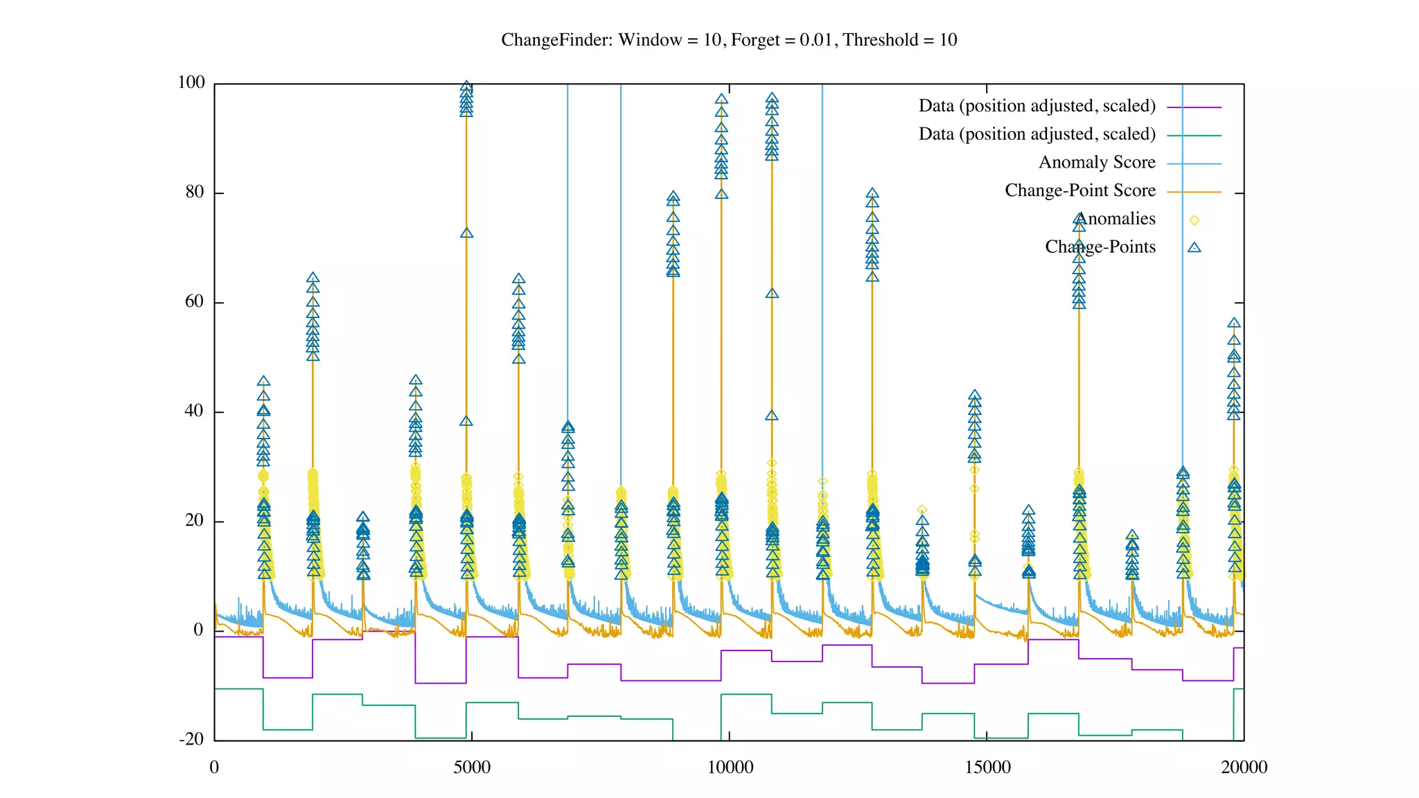
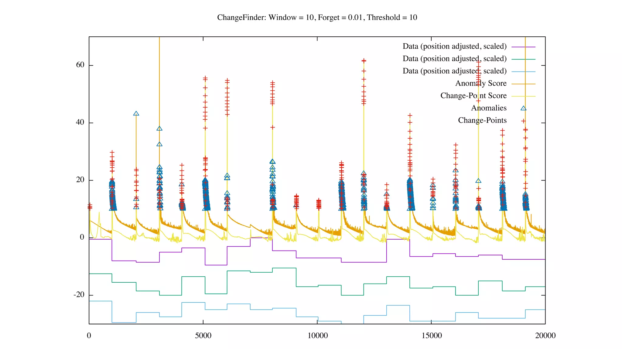
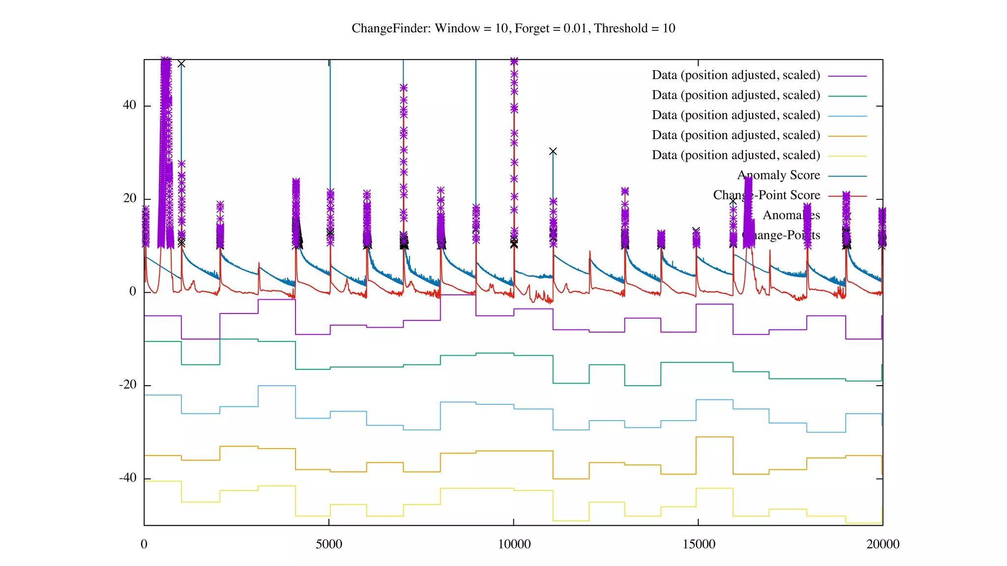
Status of ChangeFinder within Hivemall
• No pull request yet
• https://github.com/L3Sota/hivemall/tree/feature/cf_sdar_focused
• Mostly complete but some issues remain with detection accuracy, esp. at
higher dimensions
• cf_detect(array<double> x[, const string options])
• ChangeFinder expects input one data point (one vector) at a time, and
automatically learns from the data in the order provided while returning
detection results.

How was Interning?
• Educational
• Eclipse
• Maven
• Java
• Contributing to an existing project
• Inspiring
• Cool people doing cool stuff, and I get to join in
• Critical
• Next steps: Code more! Get more experience!
• Shifting from “doing what I’m told” to “think what the next step is”

Spring 2016 Intern at Treasure Data

Recommended

Recommended

More Related Content

Similar to Spring 2016 Intern at Treasure Data

Similar to Spring 2016 Intern at Treasure Data (20)

Recently uploaded

Recently uploaded (20)

Spring 2016 Intern at Treasure Data

Editor's Notes