Download as PDF, PPTX
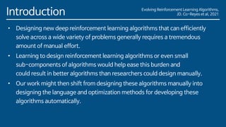
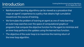
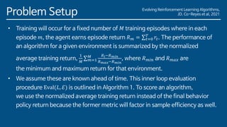
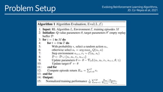
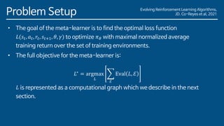
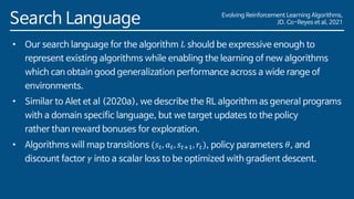
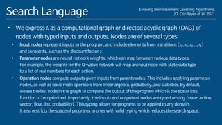

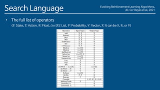
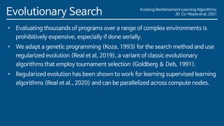
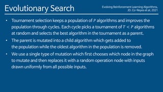
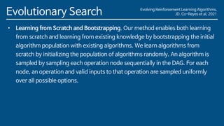
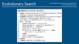
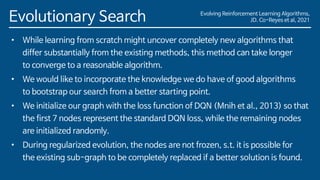
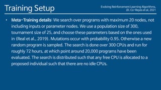
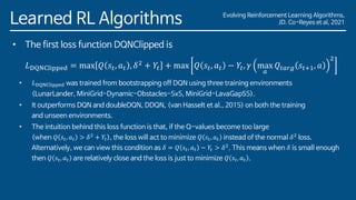
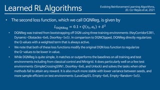

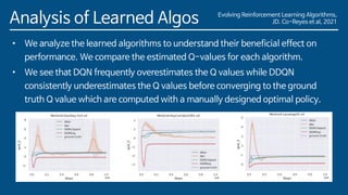
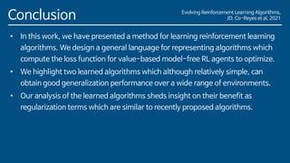
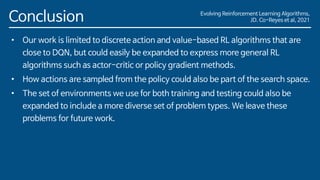


The document discusses the development of a new meta-learning framework for designing reinforcement learning algorithms automatically, aiming to reduce manual efforts while enabling the creation of domain-agnostic, efficient algorithms. The authors propose a search language based on genetic programming to express symbolic loss functions and utilize regularized evolution for optimizing these algorithms across various environments. They demonstrate that this approach successfully outperforms existing algorithms by learning two new algorithms that generalize well to unseen environments.


![[RLKorea] <하스스톤> 강화학습 환경 개발기](https://cdn.slidesharecdn.com/ss_thumbnails/rlkorea-hearthstonesimulationforreinforcementlearningver1-190826145318-thumbnail.jpg?width=640&height=640&fit=bounds)
![[NDC 2019] 하스스톤 강화학습 환경 개발기](https://cdn.slidesharecdn.com/ss_thumbnails/ndc19hearthstonedevelopmentforreinforcementlearningverfinal-190426141251-thumbnail.jpg?width=640&height=640&fit=bounds)

![[델리만주] 대학원 캐슬 - 석사에서 게임 프로그래머까지](https://cdn.slidesharecdn.com/ss_thumbnails/asdf-190219141801-thumbnail.jpg?width=640&height=640&fit=bounds)


![[NDC 2018] 유체역학 엔진 개발기](https://cdn.slidesharecdn.com/ss_thumbnails/ndc18fluidenginedevelopmentverfinal-180427164620-thumbnail.jpg?width=640&height=640&fit=bounds)


![[9XD] Introduction to Computer Graphics](https://cdn.slidesharecdn.com/ss_thumbnails/introductiontocomputergraphics-170415035926-thumbnail.jpg?width=640&height=640&fit=bounds)

![[제1회 시나브로 그룹 오프라인 밋업] 개발자의 자존감](https://cdn.slidesharecdn.com/ss_thumbnails/random-170325145337-thumbnail.jpg?width=640&height=640&fit=bounds)


