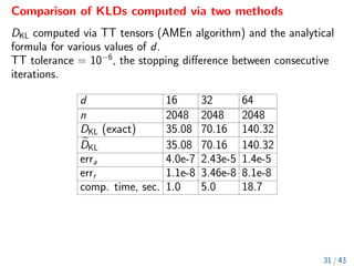
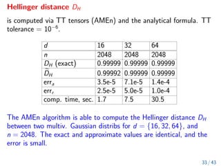
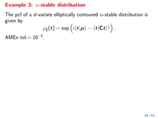
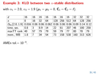
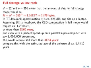
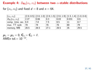
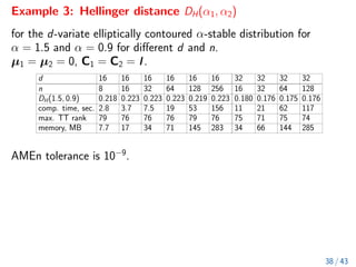
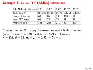
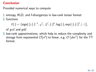
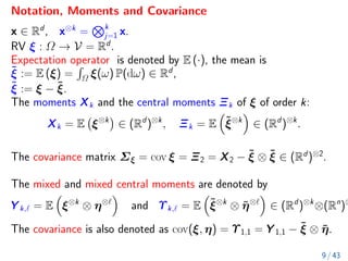
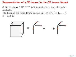
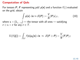
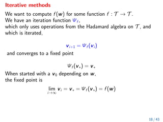
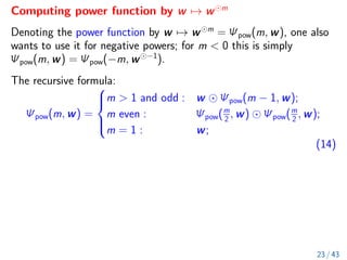
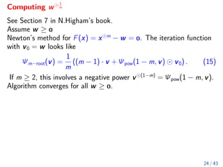
The document discusses methods for computing f-divergences and distances of high-dimensional probability density functions (PDFs), focusing on when PDFs are unknown. It includes the theoretical background, algorithms for computation, applications in stochastic partial differential equations, and various methods such as tensor formats and numerical techniques. The document also presents discrete approximations for divergences, computational algorithms, and iterative methods for evaluating functions of tensors.


![Connection of pcf and pdf
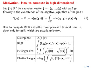
The probability characteristic function (pcf ) ϕξ defined:
ϕξ(t) := E (exp(ihξ|ti)) :=
Z
Rd
pξ(y) exp(ihy|ti) dy =: F[d]
(pξ)(t),
where t = (t1, t2, ..., td) ∈ Rd
,
hy|ti =
Pd
j=1 yjtj, and
F[d]
is the probabilist’s d-dimensional Fourier transform.
pξ(y) =
1
(2π)d
Z
Rd
exp(−iht|yi)ϕξ(t) dt = F[−d]
(ϕξ)(y). (4)
5 / 43](https://image.slidesharecdn.com/litvinenkorwthuqseminartalk-221025223214-89606317/85/Litvinenko_RWTH_UQ_Seminar_talk-pdf-6-320.jpg)
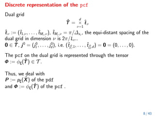
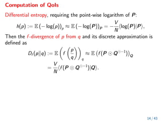
![Discrete low-rank representation of pcf
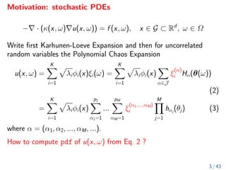
We try to find an approximation
ϕξ(t) ≈ e
ϕξ(t) =
R
X
`=1
d
O
ν=1
ϕ`,ν(tν), (5)
where the ϕ`,ν(tν) are one-dimensional functions.
Then we can get
pξ(y) ≈ e
pξ(y) = F[−d]
(e
ϕξ)y =
R
X
`=1
d
O
ν=1
F−1
1 (ϕ`,ν)(yν),
where F−1
1 is the one-dimensional inverse Fourier transform.
6 / 43](https://image.slidesharecdn.com/litvinenkorwthuqseminartalk-221025223214-89606317/85/Litvinenko_RWTH_UQ_Seminar_talk-pdf-7-320.jpg)
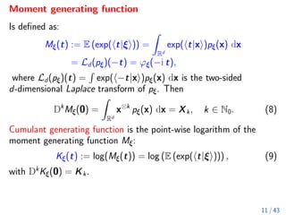
![Higher order moments
(−i ∂tk
) ϕξ(t) =
R
Rd xk exp(iht|xi)pξ(x) dx = F[d]
(xkpξ(x)) (t).
Further, denoting the tensor of k-th derivatives by
Dk
ϕξ(t) =
∂k
∂ti1
... ∂tik
ϕξ(t)
, and
(−i)k
Dk
ϕξ(0) =
Z
Rd
x⊗k
pξ(x) dx = F[d]
x⊗k
pξ(x)
(0) = Xk
(6)
Second characteristic function (cumulant generating function) whose
derivative tensors of order k are essentially the cumulants Kk of ξ, is
defined as the point-wise logarithm of the pcf :
χξ(t) := log(ϕξ(t)) = log (E (exp(iht|ξi))) , (7)
with (−i)k
Dk
χξ(0) =: Kk.
10 / 43](https://image.slidesharecdn.com/litvinenkorwthuqseminartalk-221025223214-89606317/85/Litvinenko_RWTH_UQ_Seminar_talk-pdf-11-320.jpg)
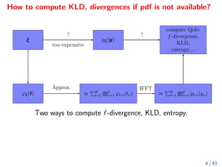
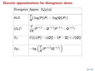
![List of some typical divergences and distances.
Divergence D•(pkq)
KLD — DKL:
Z
(log(p(x)/q(x))) p(x) dx = Ep(log(p/q))
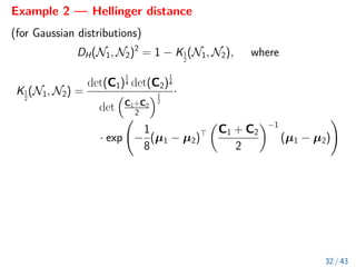
Hellinger,(DH)2
:
1
2
Z q
p(x) −
q
q(x)
2
dx
Bregman, Dφ:
Z
[(φ(p(x)) − φ(q(x))) − (p(x) − q(x))φ0
(q(x))] dx
Bhattach., DBh: − log
Z q
(p(x)q(x)) dx
15 / 43](https://image.slidesharecdn.com/litvinenkorwthuqseminartalk-221025223214-89606317/85/Litvinenko_RWTH_UQ_Seminar_talk-pdf-16-320.jpg)
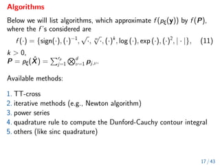
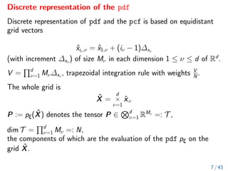
![Computing pointwise
√
w via Newton-Schulz iteration
Let F(x) := x 2
− w = 0.
An alternative is Newton-Schulz iteration, which computes
v+
∗ =
√
w = w 1/2
and v−
∗ = (
√
w) −1
= w −1/2
.
We set V 0 = [y0, z0] = [α · w, ] ∈ T 2
, and the auxiliary function
A(y, z) = 3 · − z y:
Ψ√
y
z
=
1
2
y A(y, z)
A(y, z) z
. (13)
The iteration converges to V ∗ = [v+
∗ , v−
∗ ] = [
√
y0, (
√
y0) −1
] if
k − y0k∞ 1, which can be achieved with a scaling factor
α 1/kwk∞.
As the initial iterate was scaled, the fixed point of the iteration is
v+
∗ =
√
α ·
√
w and v−
∗ = (1/
√
α) · (
√
w) −1
.
Thus the final result is
√
w = (1/
√
α)·v+
∗ and (
√
w) −1
=
√
α ·v−
∗ .
21 / 43](https://image.slidesharecdn.com/litvinenkorwthuqseminartalk-221025223214-89606317/85/Litvinenko_RWTH_UQ_Seminar_talk-pdf-22-320.jpg)
![Computing w
1
m
Auxiliary function A(y, z) = (1/m) · ((m + 1) · − z):
Ψm−root =
y
z
=
y A(y, z)
Ψpow(m, A(y, z)) z
, (16)
where yi → w − 1
m and zi → w
1
m .
The starting values are V 0 = [y0, z0] = [α · , (α)m
w] ∈ T 2
,
with α (kwk∞/
√
2)− 1
m .
For scaling purposes it is best used with m = 2k
.
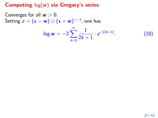
25 / 43](https://image.slidesharecdn.com/litvinenkorwthuqseminartalk-221025223214-89606317/85/Litvinenko_RWTH_UQ_Seminar_talk-pdf-26-320.jpg)
![Computing w
1
m
Another way of computing the m-th root is Tsai’s algorithm(Tsai’88,
Lorin’21), which uses the auxiliary function
B(y) = (2 · + (m − 2) · y) ( + (m − 1) · y) −1
:
ΨTsai =
y
z
=
y Ψpow(m, B(y))
z (B(y))
, (17)
with starting value V 0 = [w, ]. Then zi → w
1
m .
26 / 43](https://image.slidesharecdn.com/litvinenkorwthuqseminartalk-221025223214-89606317/85/Litvinenko_RWTH_UQ_Seminar_talk-pdf-27-320.jpg)