The document discusses data sparse approximation techniques related to the Karhunen-Loève expansion, focusing on numerical methods, eigenvalue problems, and the covariance structure of random fields. It explores applications such as solving stochastic partial differential equations and higher-order moments, employing methods like FFT, hierarchical matrices, and tensor approximations to achieve computational efficiency. The analysis includes examples of covariance functions and the associated computational complexity of different approximation techniques.

1. Data sparse approximation of the
Karhunen-Lo`eve expansion
Alexander Litvinenko,
joint with B. Khoromskij (Leipzig) and H. Matthies(Braunschweig)
Institut f¨ur Wissenschaftliches Rechnen, Technische Universit¨at Braunschweig,
0531-391-3008, litvinen@tu-bs.de
March 5, 2008

2. Outline
Introduction
KLE
Numerical techniques
FFT
Hierarchical Matrices
Sparse tensor approximation
Application
Conclusion

3. Outline
Introduction
KLE
Numerical techniques
FFT
Hierarchical Matrices
Sparse tensor approximation
Application
Conclusion

4. Stochastic PDE
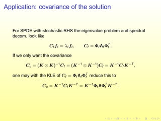
We consider
− div(κ(x, ω)∇u) = f(x, ω) in D,
u = 0 on ∂D,
with stochastic coefficients κ(x, ω), x ∈ D ⊆ Rd
and ω belongs to the
space of random events Ω.
[Babuˇska, Ghanem, Matthies, Schwab, Vandewalle, ...].
Methods and techniques:
1. Response surface
2. Monte-Carlo
3. Perturbation
4. Stochastic Galerkin

5. Examples of covariance functions [Novak,(IWS),04]
The random field requires to specify its spatial correl. structure
covf (x, y) = E[(f(x, ·) − µf (x))(f(y, ·) − µf (y))],
where E is the expectation and µf (x) := E[f(x, ·)].
Let h =
3
i=1 h2
i /ℓ2
i + d2 − d
2
, where hi := xi − yi , i = 1, 2, 3,
ℓi are cov. lengths and d a parameter.
Gaussian cov(h) = σ2
· exp(−h2
),
exponential cov(h) = σ2
· exp(−h),
spherical
cov(h) =
σ2
· 1 − 3
2
h
hr
− 1
2
h3
h3
r
for 0 ≤ h ≤ hr ,
0 for h > hr .

6. Outline
Introduction
KLE
Numerical techniques
FFT
Hierarchical Matrices
Sparse tensor approximation
Application
Conclusion

7. KLE
The spectral representation of the cov. function is
Cκ(x, y) = ∞
i=0 λi ki(x)ki (y), where λi and ki(x) are the eigenvalues
and eigenfunctions.
The Karhunen-Lo`eve expansion [Loeve, 1977] is the series
κ(x, ω) = µk (x) +
∞
i=1
λi ki (x)ξi (ω), where
ξi (ω) are uncorrelated random variables and ki are basis functions in
L2
(D).
Eigenpairs λi , ki are the solution of
Tki = λi ki, ki ∈ L2
(D), i ∈ N, where.
T : L2
(D) → L2
(D),
(Tu)(x) := D
covk (x, y)u(y)dy.

8. Outline
Introduction
KLE
Numerical techniques
FFT
Hierarchical Matrices
Sparse tensor approximation
Application
Conclusion

9. Computation of eigenpairs by FFT
If the cov. function depends on (x − y) then on a uniform tensor grid
the cov. matrix C is (block) Toeplitz.
Then C can be extended to the circulant one and the decomposition
C =
1
n
F H
ΛF (1)
may be computed like follows. Multiply (1) by F becomes
F C = ΛF ,
F C1 = ΛF1.
Since all entries of F1 are unity, obtain
λ = F C1.
F C1 may be computed very efficiently by FFT [Cooley, 1965] in
O(n log n) FLOPS.
C1 may be represented in a matrix or in a tensor format.

10. Multidimensional FFT
Lemma: The d-dim. FT F (d)
can be represented as following
F (d)
= (F
(1)
1 ⊗ I ⊗ I . . .)(I ⊗ F
(1)
2 ⊗ I . . .) . . . (I ⊗ I . . . ⊗ F
(1)
d ), (2)
and the complexity of F (d)
is O(nd
log n), where n is the number of
dofs in one direction.

11. Discrete eigenvalue problem
Let
Wij :=
k,m D
bi (x)bk (x)dxCkm
D
bj (y)bm(y)dy,
Mij =
D
bi (x)bj (x)dx.
Then we solve
W fh
ℓ = λℓMfh
ℓ , where W := MCM
Approximate C in
◮ low rank format
◮ the H-matrix format
◮ sparse tensor format
and use the Lanczos method to compute m largest eigenvalues.

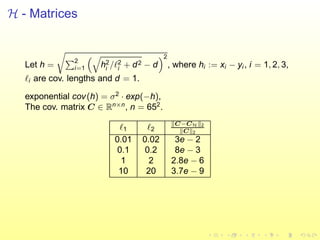
12. Examples of H-matrix approximates of
cov(x, y) = e−2|x−y|
[Hackbusch et al. 99]
25 20
20 20
20 16
20 16
20 20
16 16
20 16
16 16
4 4
20 4 32
4 4
16 4 32
4 20
4 4
4 16
4 4
32 32
20 20
20 20 32
32 32
4 3
4 4 32
20 4
16 4 32
32 4
32 32
4 32
32 32
32 4
32 32
4 4
4 4
20 16
4 4
32 32
4 32
32 32
32 32
4 32
32 32
4 32
20 20
20 20 32
32 32
32 32
32 32
32 32
32 32
32 32
32 32
4 4
4 4
20 4 32
32 32 4
4 4
32 4
32 32 4
4 4
32 32
4 32 4
4 4
32 32
32 32 4
4
4 20
4 4 32
32 32
4 4
4
32 4
32 32
4 4
4
32 32
4 32
4 4
4
32 32
32 32
4 4
20 20
20 20 32
32 32
4 4
20 4 32
32 32
4 20
4 4 32
32 32
20 20
20 20 32
32 32
32 4
32 32
32 4
32 32
32 4
32 32
32 4
32 32
32 32
4 32
32 32
4 32
32 32
4 32
32 32
4 32
32 32
32 32
32 32
32 32
32 32
32 32
32 32
32 32
4 4
4 4 44 4
20 4 32
32 32
32 4
32 32
4 32
32 32
32 4
32 32
4 4
4 4
4 4
4 4 4
4 4
32 4
32 32 4
4 4
4 4
4 4
4 4 4
4
32 4
32 32
4 4
4 4
4 4
4 4
4 4 4
32 4
32 32
32 4
32 32
32 4
32 32
32 4
32 32
4 4
4 4
4 4
4 4
4 20
4 4 32
32 32
4 32
32 32
32 32
4 32
32 32
4 32
4
4 4
4 4
4 4
4 4
4 4
32 32
4 32 4
4
4 3
4 4
4 4
4 4
4
32 32
4 32
4 4
4
4 4
4 4
4 4
4 4
32 32
4 32
32 32
4 32
32 32
4 32
32 32
4 32
4
4 4
4 4
20 20
20 20 32
32 32
32 32
32 32
32 32
32 32
32 32
32 32
4 4
20 4 32
32 32
32 4
32 32
4 32
32 32
32 4
32 32
4 20
4 4 32
32 32
4 32
32 32
32 32
4 32
32 32
4 32
20 20
20 20 32
32 32
32 32
32 32
32 32
32 32
32 32
32 32
4 4
32 32
32 32 4
4 4
32 4
32 32 4
4 4
32 32
4 32 4
4 4
32 32
32 32 4
4
32 32
32 32
4 4
4
32 4
32 32
4 4
4
32 32
4 32
4 4
4
32 32
32 32
4 4
32 32
32 32
32 32
32 32
32 32
32 32
32 32
32 32
32 4
32 32
32 4
32 4
32 4
32 32
32 4
32 4
32 32
4 32
32 32
4 32
32 32
4 4
32 32
4 4
32 32
32 32
32 32
32 32
32 32
32 32
32 32
32 32
25 11
11 20 12
13
20 11
9 16
13
13
20 11
11 20 13
13 32
13
13
20 8
10 20 13
13 32 13
13
32 13
13 32
13
13
20 11
11 20 13
13 32 13
13
20 10
10 20 12
12 32
13
13
32 13
13 32 13
13
32 13
13 32
13
13
20 11
11 20 13
13 32 13
13
32 13
13 32
13
13
20 9
9 20 13
13 32 13
13
32 13
13 32
13
13
32 13
13 32 13
13
32 13
13 32
13
13
32 13
13 32 13
13
32 13
13 32
Figure: H-matrix approximations ∈ Rn×n
, n = 322
, with standard (left) and
weak (right) admissibility block partitionings. The biggest dense (dark) blocks
∈ Rn×n
, max. rank k = 4 left and k = 13 right.

13. H - Matrices
Comp. complexity is O(kn log n) and storage O(kn log n).
To assemble low-rank blocks use ACA [Bebendorf, Tyrtyshnikov].
Dependence of the computational time and storage requirements of
CH on the rank k, n = 322
.
k time (sec.) memory (MB) C−CH 2
C 2
2 0.04 2e + 6 3.5e − 5
6 0.1 4e + 6 1.4e − 5
9 0.14 5.4e + 6 1.4e − 5
12 0.17 6.8e + 6 3.1e − 7
17 0.23 9.3e + 6 6.3e − 8
The time for dense matrix C is 3.3 sec. and the storage 1.4e + 8 MB.

14. H - Matrices
Let h =
2
i=1 h2
i /ℓ2
i + d2 − d
2
, where hi := xi − yi , i = 1, 2, 3,
ℓi are cov. lengths and d = 1.
exponential cov(h) = σ2
· exp(−h),
The cov. matrix C ∈ Rn×n
, n = 652
.
ℓ1 ℓ2
C−CH 2
C 2
0.01 0.02 3e − 2
0.1 0.2 8e − 3
1 2 2.8e − 6
10 20 3.7e − 9

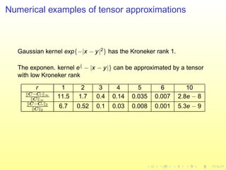
15. Exponential Singularvalue decay [see also Schwab et
al.]
0 100 200 300 400 500 600 700 800 900 1000
0
100
200
300
400
500
600
700
0 100 200 300 400 500 600 700 800 900 1000
0
1
2
3
4
5
6
7
8
9
10
x 10
4
0 100 200 300 400 500 600 700 800 900 1000
0
200
400
600
800
1000
1200
1400
1600
1800
0 100 200 300 400 500 600 700 800 900 1000
0
0.5
1
1.5
2
2.5
x 10
5
0 100 200 300 400 500 600 700 800 900 1000
0
50
100
150
0 100 200 300 400 500 600 700 800 900 1000
0
0.5
1
1.5
2
2.5
3
3.5
4
x 10
4

16. Sparse tensor decompositions of kernels
cov(x, y) = cov(x − y)
We want to approximate C ∈ RN×N
, N = nd
by
Cr =
r
k=1 V 1
k ⊗ ... ⊗ V d
k such that C − Cr ≤ ε.
The storage of C is O(N2
) = O(n2d
) and the storage of Cr is O(rdn2
).
To define V i
k use e.g. SVD.
Approximate all V i
k in the H-matrix format and become HKT format.
See basic arithmetics in [Hackbusch, Khoromskij, Tyrtyshnikov].
Assume f(x, y), x = (x1, x2), y = (y1, y2), then the equivalent approx.
problem is f(x1, x2; y1, y2) ≈
r
k=1 Φk (x1, y1)Ψk (x2, y2).

17. Numerical examples of tensor approximations
Gaussian kernel exp{−|x − y|2
} has the Kroneker rank 1.
The exponen. kernel e{
− |x − y|} can be approximated by a tensor
with low Kroneker rank
r 1 2 3 4 5 6 10
C−Cr ∞
C ∞
11.5 1.7 0.4 0.14 0.035 0.007 2.8e − 8
C−Cr 2
C 2
6.7 0.52 0.1 0.03 0.008 0.001 5.3e − 9

18. Outline
Introduction
KLE
Numerical techniques
FFT
Hierarchical Matrices
Sparse tensor approximation
Application
Conclusion

19. Application: covariance of the solution
For SPDE with stochastic RHS the eigenvalue problem and spectral
decom. look like
Cf fℓ = λℓfℓ, Cf = Φf Λf ΦT
f .
If we only want the covariance
Cu = (K ⊗ K)−1
Cf = (K−1
⊗ K−1
)Cf = K−1
Cf K−T
,
one may with the KLE of Cf = Φf Λf ΦT
f reduce this to
Cu = K−1
Cf K−T
= K−1
Φf ΛΦT
f K−T
.

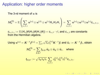
20. Application: higher order moments
Let operator K be deterministic and
Ku(θ) =
α∈J
Ku(α)
Hα(θ) = ˜f(θ) =
α∈J
f(α)
Hα(θ), with
u(α)
= [u
(α)
1 , ..., u
(α)
N ]T
. Projecting onto each Hα obtain
Ku(α)
= f(α)
.
The KLE of f(θ) is
f(θ) = f +
ℓ
λℓφℓ(θ)fl =
ℓ α
λℓφ
(α)
ℓ Hα(θ)fl
=
α
Hα(θ)f(α)
,
where f(α)
= ℓ
√
λℓφ
(α)
ℓ fl .

21. Application: higher order moments
The 3-rd moment of u is
M
(3)
u = E


α,β,γ
u(α)
⊗ u(β)
⊗ u(γ)
HαHβHγ

 =
α,β,γ
u(α)
⊗u(β)
⊗u(γ)
cα,β,γ,
cα,β,γ := E (Hα(θ)Hβ(θ)Hγ(θ)) = cα,β · γ!, and cα,β are constants
from the Hermitian algebra.
Using u(α)
= K−1
f(α)
= ℓ
√
λℓφ
(α)
ℓ K−1
fl and uℓ := K−1
fℓ, obtain
M
(3)
u =
p,q,r
tp,q,r up ⊗ uq ⊗ ur , where
tp,q,r := λpλqλr
α,β,γ
φ
(α)
p φ
(β)
q φ
(γ)
r cα,βγ.

22. Outline
Introduction
KLE
Numerical techniques
FFT
Hierarchical Matrices
Sparse tensor approximation
Application
Conclusion

23. Conclusion
◮ Covariance matrices allow data sparse low-rank approximations.
◮ With application of H-matrices
◮ we extend the class of covariance functions to work with,
◮ allows non-regular discretisations of the cov. function on large
spatial grids.
◮ Application of sparse tensor product allows computation of k-th
moments.

24. Plans for Feature
1. Convergence of the Lanczos method with H-matrices
2. Implement sparse tensor vector product for the Lanczos method
3. HKT idea for d ≥ 3 dimensions

25. Thank you for your attention!
Questions?