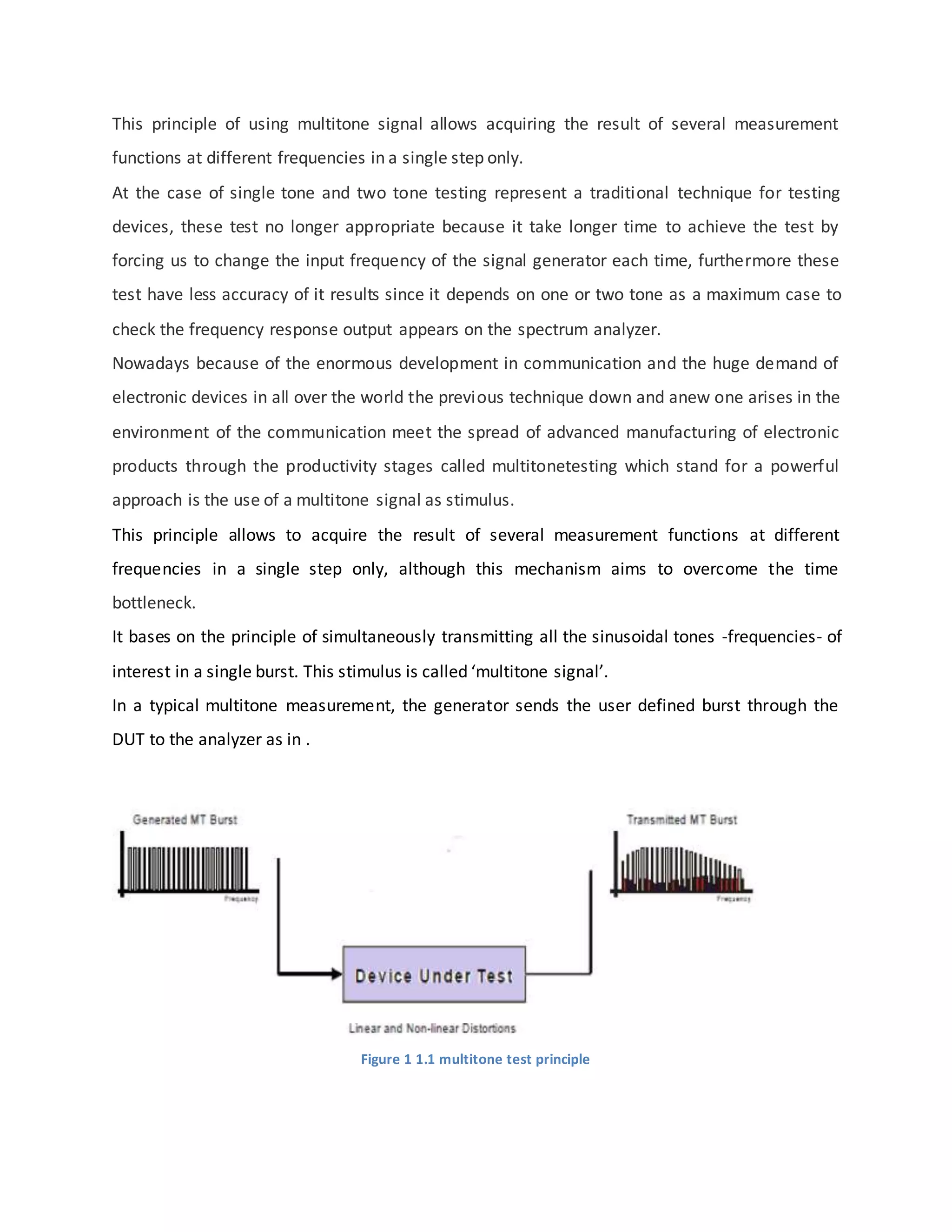
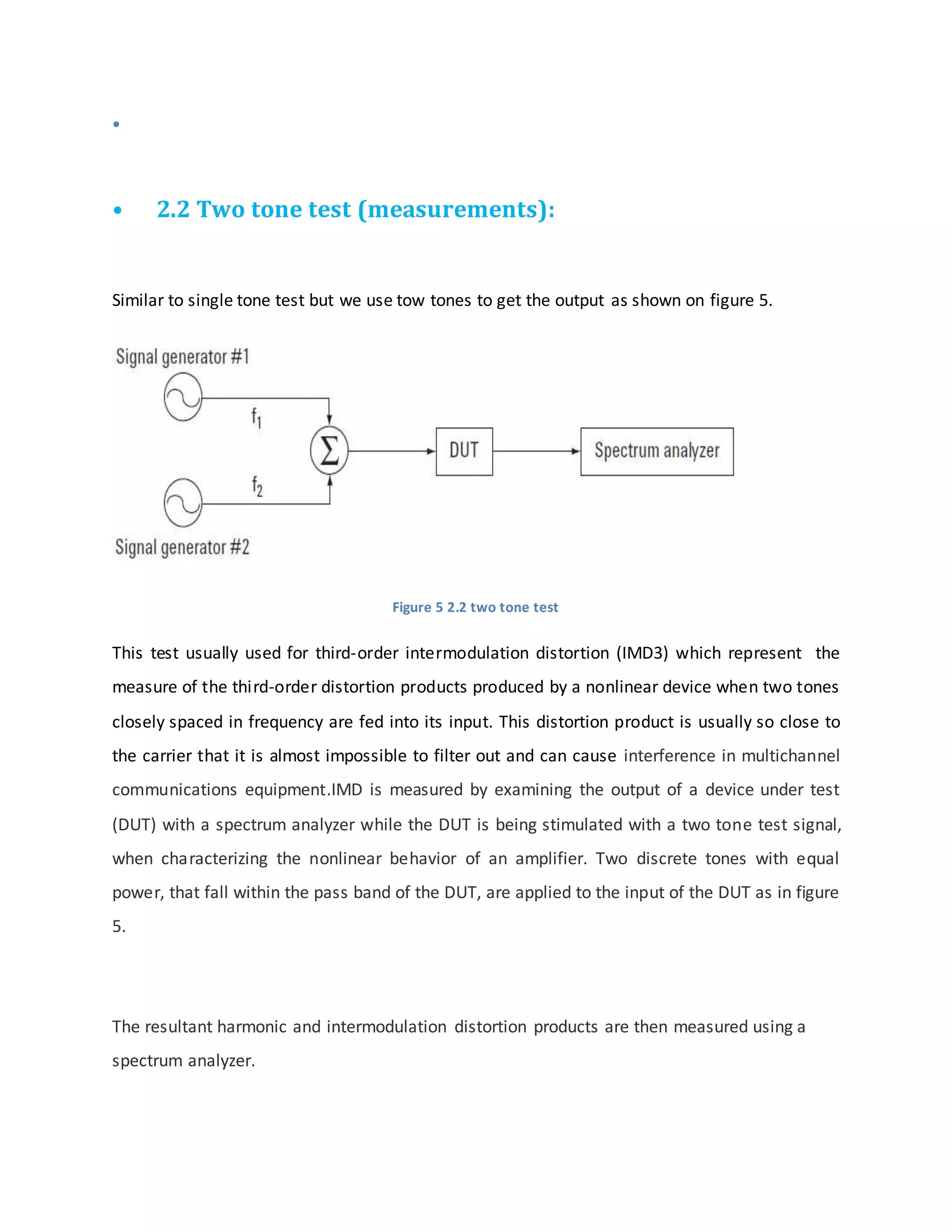
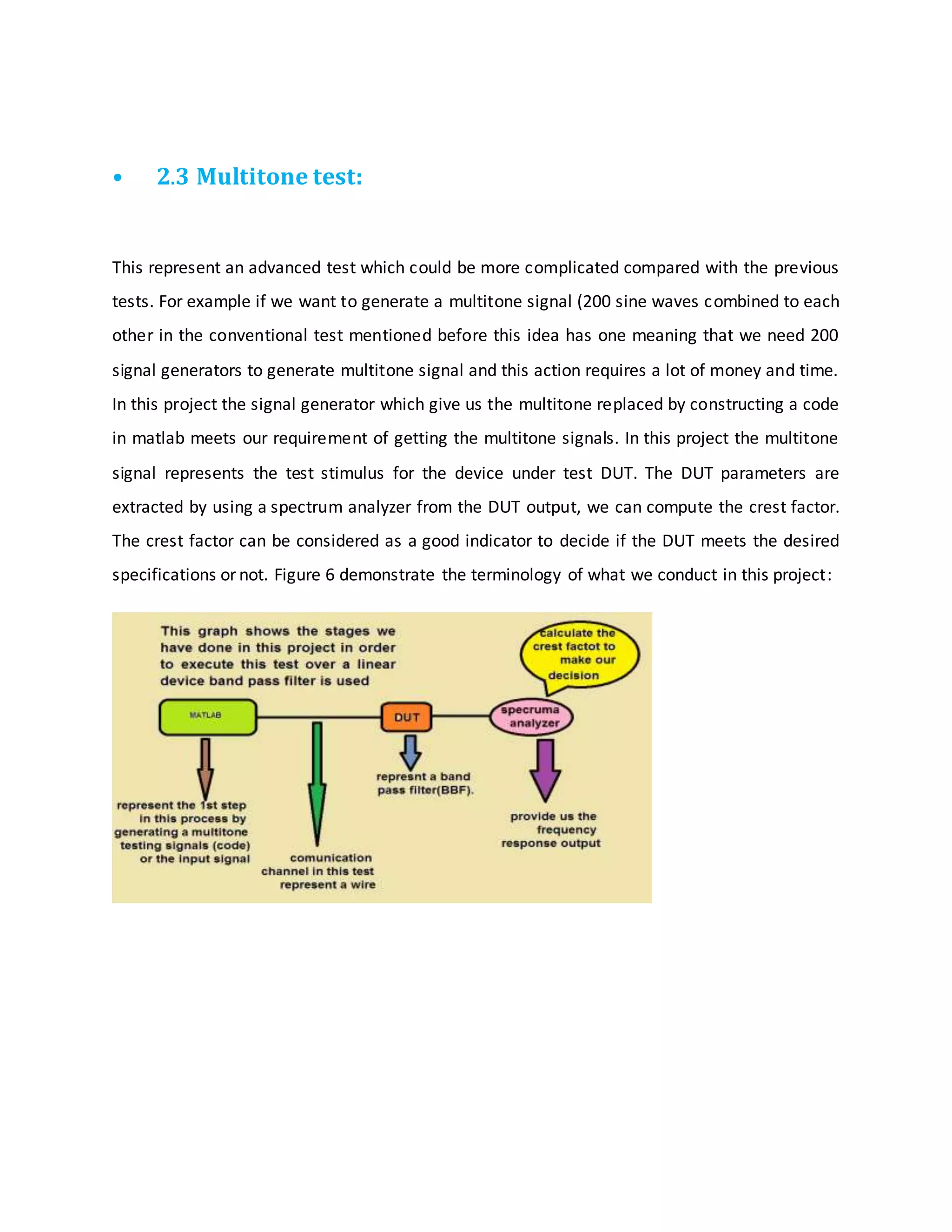
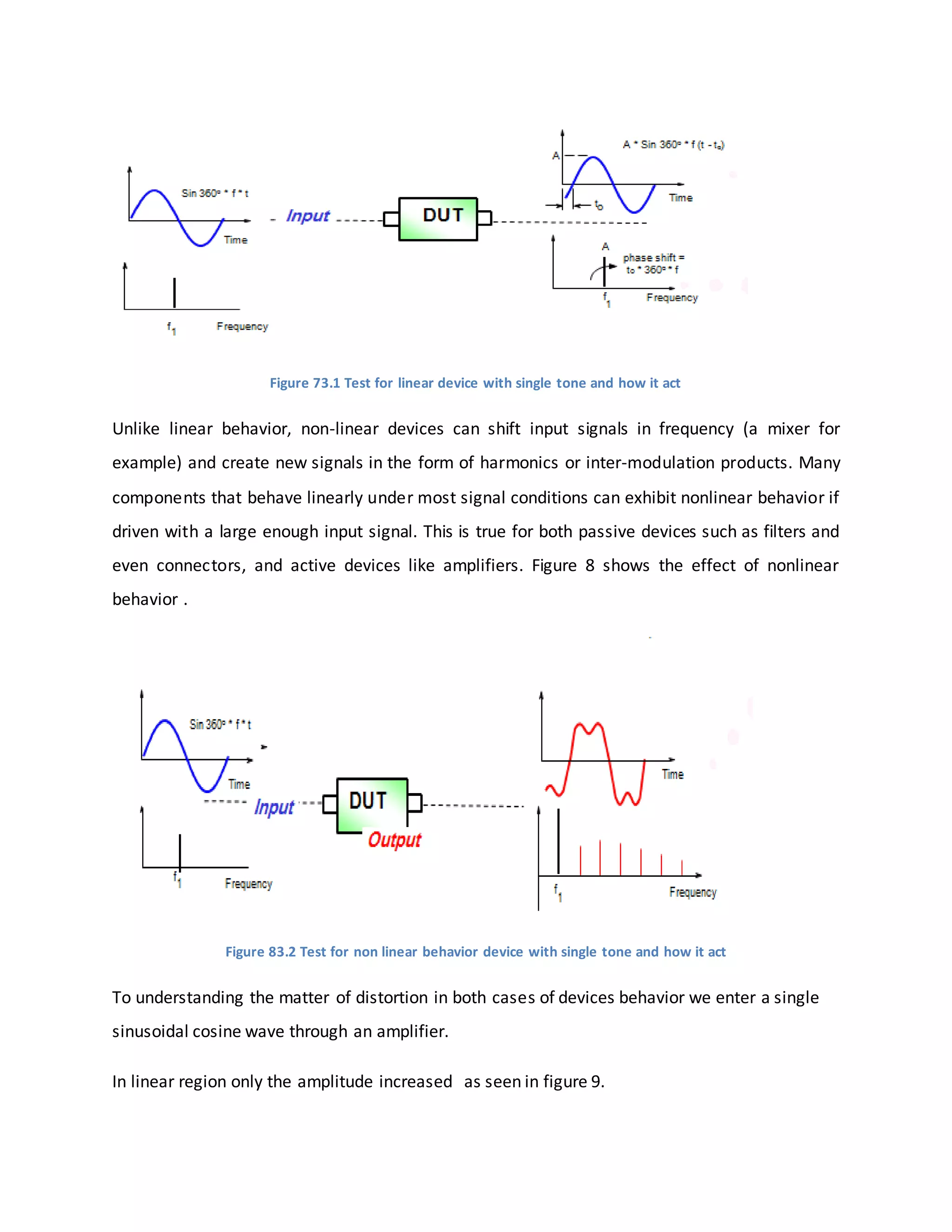
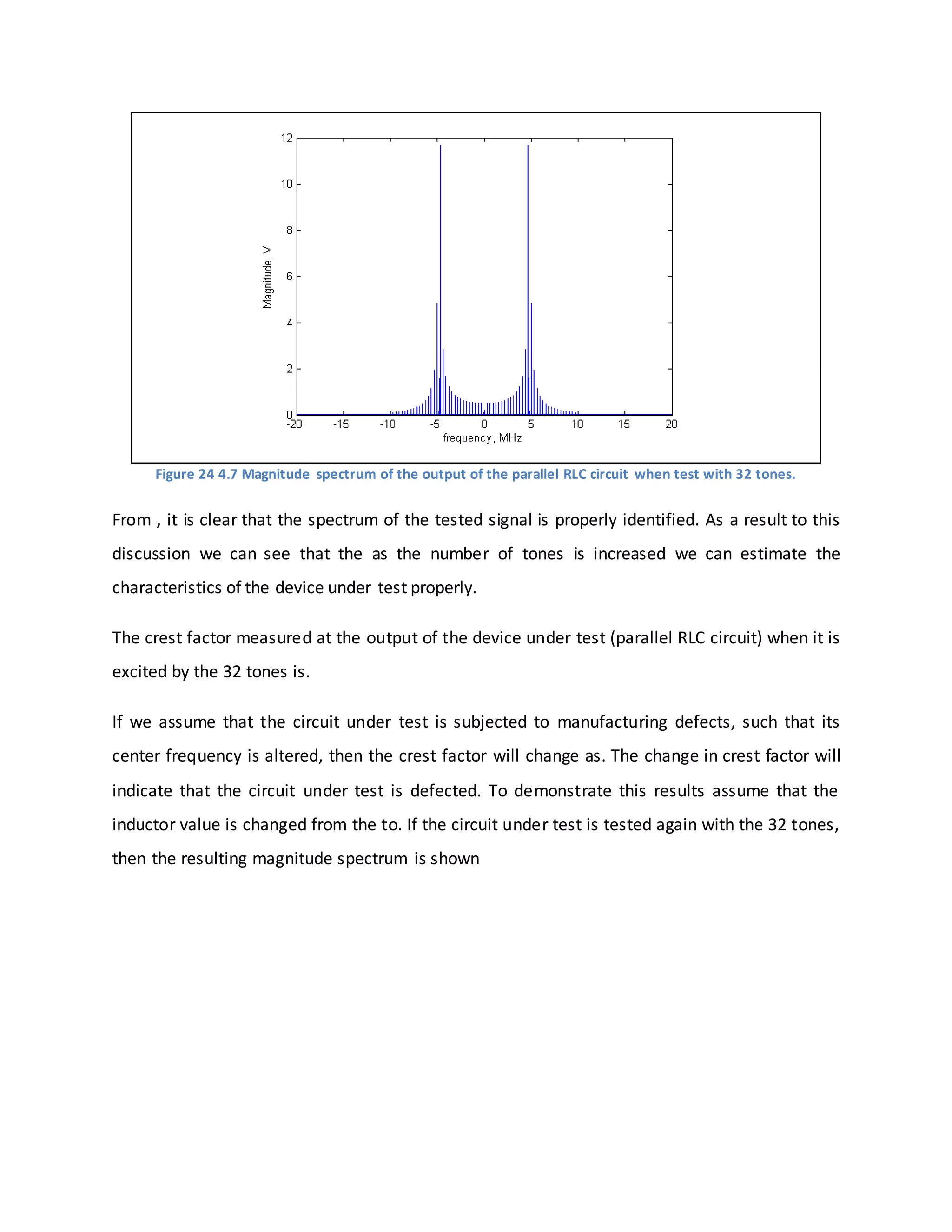
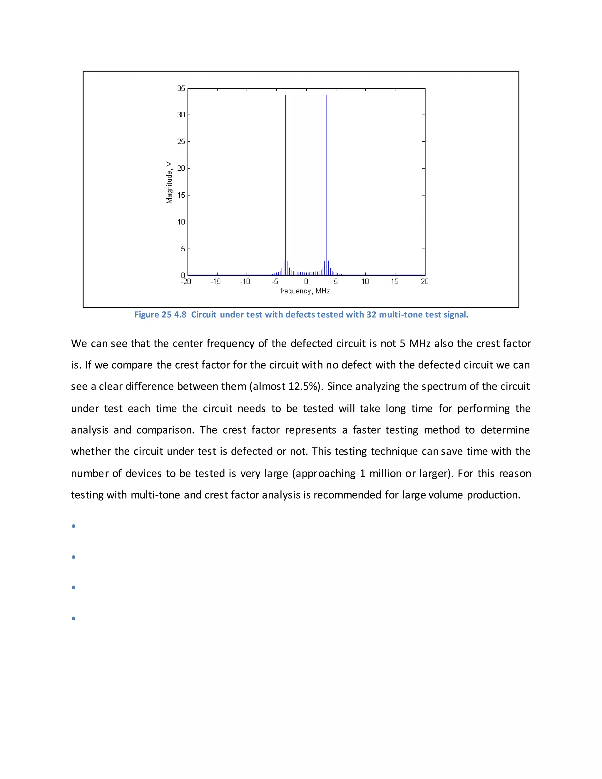
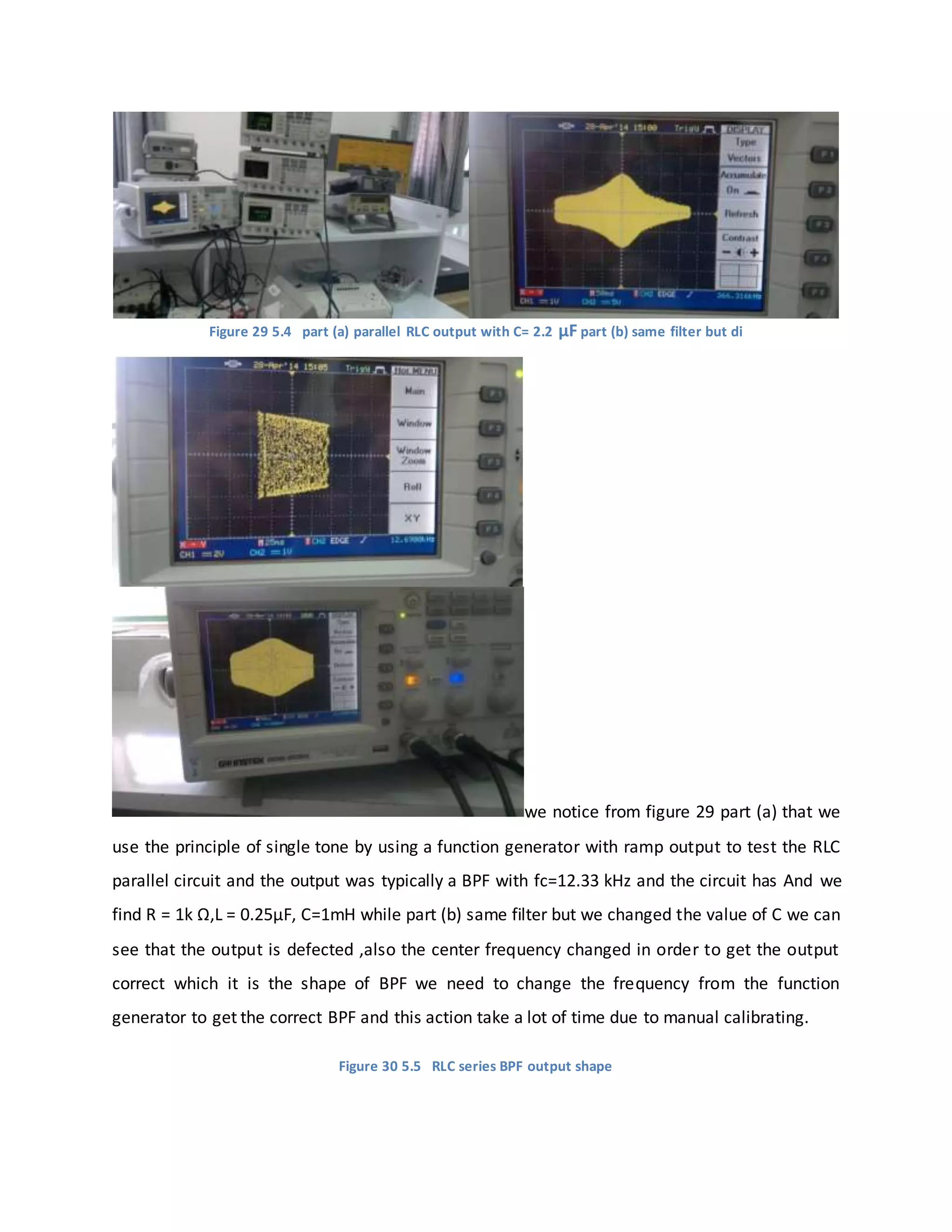
This document provides a summary of multitone testing techniques for electronic devices. It begins with an overview of how multitone testing allows acquiring measurement results from multiple frequencies simultaneously, unlike traditional single-tone and two-tone testing which require changing the input frequency each time. It then discusses some key problems that necessitate multitone testing such as reducing time and cost. Finally, it provides motivations for carrying out multitone testing research such as gaining experience in technical writing and learning newer testing methods used in manufacturing. The document contains figures illustrating multitone signals and how they are used to test devices.


![Uint32 fs = DSK6713_AIC23_FREQ_96KHZ; //set sampling rate
short loop = 0; //table index
short gain = 10; //gain factor
interrupt void c_int11() //interrupt service routine
{
short sample_data;
output_sample(multitone[loop]); //output data
if(++loop>128) loop=0; //reset the loop when all samples are sent to the output
return;
}
void main()
{
comm_intr(); //init DSK, codec, McBSP
while(1); //infinite loop
} //end of main
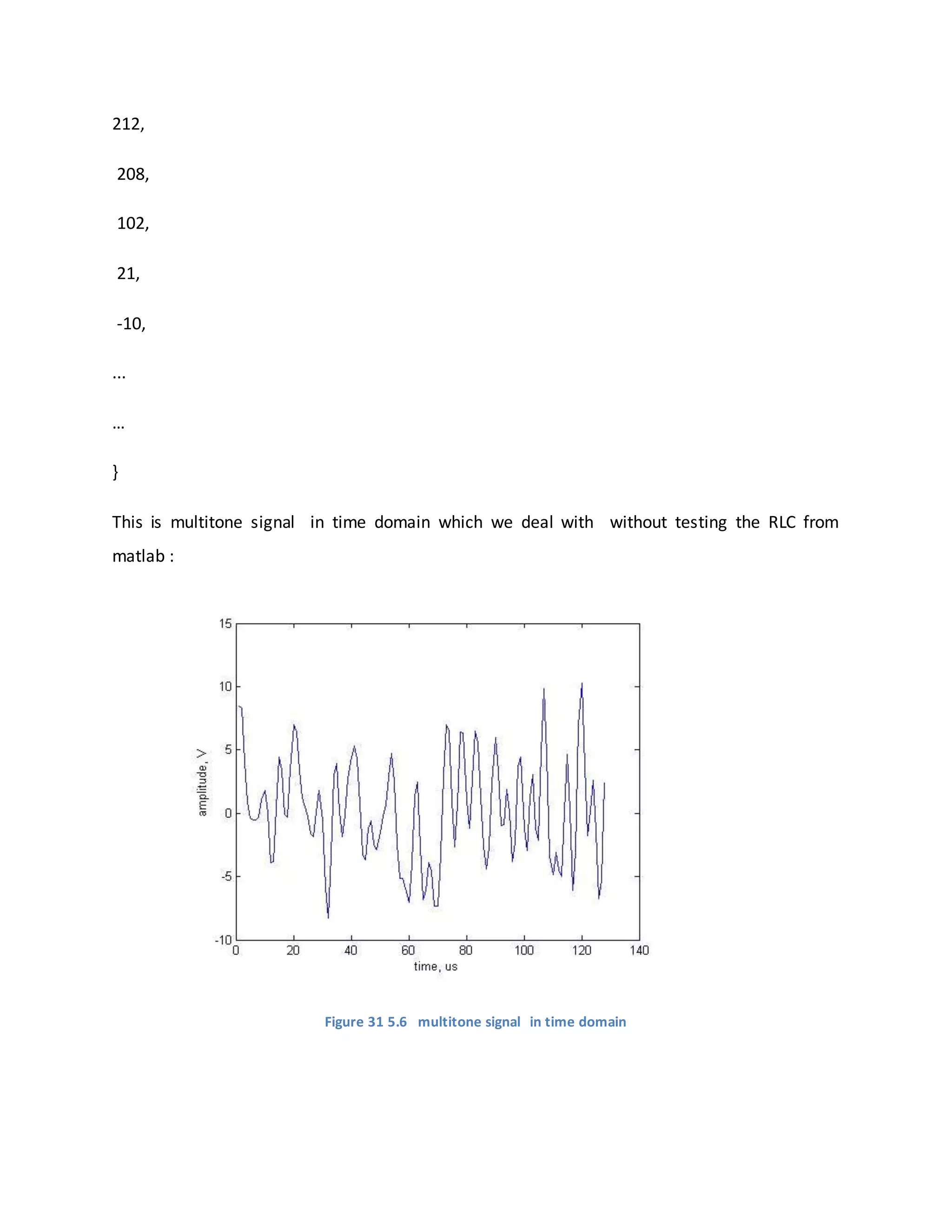
After that we take a vector contains many sample and represent the number of sample which
we want to take in our consideration to get the multitone signal to be able to check the band
bass filter .
The vector could be like that :
short multitone[]={](https://image.slidesharecdn.com/multi-tonetest-160930054002/75/Multi-tone-test-40-2048.jpg)


![•
•
•
•
•
•
•
• Chapter 6
• References
[1]. KLIPPEL GmbH. http://www.klippel.de/measurements/nonlinear-distortion/multi-tone-
distortion.html. KLIPPEL GmbH in Dresden/Germany. Oct. 2006 .
[2]. Agilent Technologies. Two-tone and Multitone Personalities,Application Note 1410. USA :
Agilent Technologies, February 6, 2003.
[3]. Generation and Conditioning . USA : Agilent Technologies, December 2002.](https://image.slidesharecdn.com/multi-tonetest-160930054002/75/Multi-tone-test-49-2048.jpg)
![[4]. NTi Audio AG. Comparing Conventiona lvs. Multitone Testing,A2 . Rapid Test.
Liechtenstein : NTi Audio AG, Mar. 2000.
[5]. Alan V.Oppenheim, Ronald W.Schafer,Joun R.Buck. Discrete-Time Signal Processing .
Upper saddle river,New Jersey : Prentice-Hall,Inc., 1999.
[6]. NTI AG. Multitone Testing,RAPID-TEST Applications. FL-9494 Schaan,Liechtenstein : NTI AG,
Mar. 2000.
[7]. José Carlos Pedro, Nuno Borges Carvalho. Intermodulation Distortion in Microwave and
Wireless Circuits. 2003.
• Chapter 7
• Appendices
%function[waveform]=mtpr_input(bin_start,bin_stop,sample_size,samp_freq,max_PAR)
clear all
clc
%for z=1:100,
clear x
tic](https://image.slidesharecdn.com/multi-tonetest-160930054002/75/Multi-tone-test-50-2048.jpg)
![fcarrier = 10e6; % Frequency of the RF carrier 1 GHz
A = 5; % The perak amplitude of the test signal
sample_size=2^16; % Number of samples taken for simulation
samp_freq=4*fcarrier;
N_Tones=256;
% bin_start=33;
% bin_stop=256;
% max_PAR=16;
% missing=[48 72 96 120 144 168 192 216 240];
% Generating tone frequencies
freq=(fcarrier/N_Tones)*(1:256);
% m=0;
% for k=1:N_Tones,
% freq(k)=m+fcarrier/N_Tones;
% m=freq(k);
% num_tones(k)=k;
% end
%**********************************************************************
%**********************************************************************
%generation phases
thetha(1:N_Tones)=0.6+sqrt(pi)*randn(1,N_Tones);
%%%%%%%%%%%%%%%%%%%%%%%%%%%%
%thetha(1:N_Tones)=0;
%load('thetha.txt')
%generatin amplitudes
amp=ones(1,N_Tones);](https://image.slidesharecdn.com/multi-tonetest-160930054002/75/Multi-tone-test-51-2048.jpg)


![% power_timedomain = sum(abs(modu).^2)/length(modu); % This equation is
intended to compute the rms of a given signal
% poervector=sqrt(power_timedomain)*ones(1,length(modu));
% Crest_Factor=max(modu)/sqrt(power_timedomain); % This equation is used to
compute the crest factor
% CFvector=Crest_Factor*ones(1,length(modu)); % Create a vector to hold
multiple values of the crest factor
% plot(CFvector);
% hold on
% plot(poervector);
% hold off
% save('C:UsersLauraDocumentsMATLABnoisy_signal_GHz.txt', 'x', '-ascii');
l=1*150e-9;
c=1*6.7e-9;
r=10e3;
num=1;
den=[l*c l/r 1];
[numd,dend] = bilinear(num,den,samp_freq)
y=filter(numd,dend,x);
freq_y=fftshift(fft(y)/sample_size);
plot(1/fcarrier*samp_freq*linspace(-5,5,sample_size),abs(freq_y(1:sample_size)));
% These statments are used to compute the crest factor based on the
% avergaepower of the signal
power_timedomain = sum(abs(y).^2)/length(y); % This equation is intended to
compute the rms of a given signal
poervector=sqrt(power_timedomain)*ones(1,length(y));
Crest_Factor=max(y)/sqrt(power_timedomain);
%%%%%%%%%%%%%%%%%%%%%%%%%%%%%%%%%%%%%%%%%%%%%%%%%%](https://image.slidesharecdn.com/multi-tonetest-160930054002/75/Multi-tone-test-55-2048.jpg)
![toc
%
% save thetha.txt thetha -ascii
% copyfile('TXA.txt',['TXA' num2str(z) '.txt']);
% copyfile('thetha.txt',['Thetha' num2str(z) '.txt']);
%end
• The code used in CCstudio
include "dsk6713_aic23.h" //supportfile forcodec,DSK#
#include "multitone.h"
Uint32 fs= DSK6713_AIC23_FREQ_96KHZ; //setsamplingrate
short loop= 0; //table index
short gain= 10; //gainfactor
interruptvoidc_int11() //interruptservice routine
{
short sample_data;
output_sample(multitone[loop]);//outputdata
if(++loop>128) loop=0; //resetthe loopwhenall samplesare senttothe output
return;
}
voidmain()](https://image.slidesharecdn.com/multi-tonetest-160930054002/75/Multi-tone-test-56-2048.jpg)
![{
comm_intr();//initDSK,codec,McBSP
while(1);//infinite loop
} //endof main
Matlab code after editing
%function[waveform]=mtpr_input(bin_start,bin_stop,sample_size,samp_freq,max_PAR)
clear all
clc
%forz=1:100,
clear x
tic
fcarrier= 24e3; % Frequencyof the RFcarrier 1 GHz
A = 5; % The perakamplitude of the testsignal
sample_size=2^7; % Numberof samplestakenforsimulation
samp_freq=4*fcarrier;
N_Tones=32;
% bin_start=33;
% bin_stop=256;
% max_PAR=16;
% missing=[4872 96 120 144 168 192 216 240];
% Generatingtone frequencies
freq=(fcarrier/N_Tones)*(1:256);
% m=0;](https://image.slidesharecdn.com/multi-tonetest-160930054002/75/Multi-tone-test-57-2048.jpg)


![% power_timedomain=sum(abs(modu).^2)/length(modu); % Thisequationisintendedto
compute the rms of a givensignal
% poervector=sqrt(power_timedomain)*ones(1,length(modu));
% Crest_Factor=max(modu)/sqrt(power_timedomain); % This equationisusedtocompute
the crest factor
% CFvector=Crest_Factor*ones(1,length(modu)); % Create a vectorto holdmultiple
valuesof the crestfactor
% plot(CFvector);
% holdon
% plot(poervector);
% holdoff
% save('C:UsersLauraDocumentsMATLABnoisy_signal_GHz.txt','x','-ascii');
l=2*150e-9;
c=1*6.7e-9;
r=10e3;
num=1;
den=[l*cl/r1];
[numd,dend] =bilinear(num,den,samp_freq)
y=filter(numd,dend,x);
freq_y=fftshift(fft(y)/sample_size);
plot(1/fcarrier*samp_freq*linspace(-5,5,sample_size),abs(freq_y(1:sample_size)));
xlabel('frequency,MHz');
ylabel('Magnitude,V');
% These statmentsare usedtocompute the crest factorbasedon the
% avergaepowerof the signal](https://image.slidesharecdn.com/multi-tonetest-160930054002/75/Multi-tone-test-62-2048.jpg)
![power_timedomain=sum(abs(y).^2)/length(y); % This equationisintendedtocompute the
rms of a givensignal
poervector=sqrt(power_timedomain)*ones(1,length(y));
Crest_Factor=max(y)/sqrt(power_timedomain);
%%%%%%%%%%%%%%%%%%%%%%%%%%%%%%%%%%%%%%%%%%%%%%%%%%
figure(3)
plot(x)
xlabel('time,us')
ylabel('amplitude,V')
% power_timedomain=sum(abs(x).^2)/length(x);
% Crest_Factor=max(x)/sqrt(power_timedomain);
% Crest_Factor=max(x)/sqrt(power_timedomain);
toc
%
% save thetha.txtthetha-ascii
% copyfile('TXA.txt',['TXA'num2str(z) '.txt']);
% copyfile('thetha.txt',['Thetha'num2str(z) '.txt']);
%end
i=0:length(x)-1;
desired=round(25*x);%sin(1500)addnoise=round(100*sin(2*pi*(i)*312/8000));%sin(312)
fid=fopen('multitone.h','w');%desiredsin(1500)
fprintf(fid,'shortmultitone[]={');](https://image.slidesharecdn.com/multi-tonetest-160930054002/75/Multi-tone-test-63-2048.jpg)
![fprintf(fid,'%d,n',desired(1:length(desired)-1));
fprintf(fid,'%d',desired(length(desired)));
fprintf(fid,'};n');
fclose(fid);
The sample vector of multitone
short multitone[]={212,
208,
102,
21,
-10,
-13,
-14,
-9,
28,
45,
0,
-98,
-96,
10,
111,
85,
-2,
-8,](https://image.slidesharecdn.com/multi-tonetest-160930054002/75/Multi-tone-test-64-2048.jpg)


![Multiband Transceivers - [Chapter 4] Design Parameters of Wireless Radios](https://cdn.slidesharecdn.com/ss_thumbnails/ch4-150613070934-lva1-app6892-thumbnail.jpg?width=640&height=640&fit=bounds)


![Seller Deck - Presentation [Concert L2].PPTX](https://cdn.slidesharecdn.com/ss_thumbnails/sellerdeck-presentationconcertl2-251219171156-24982daf-thumbnail.jpg?width=640&height=640&fit=bounds)


