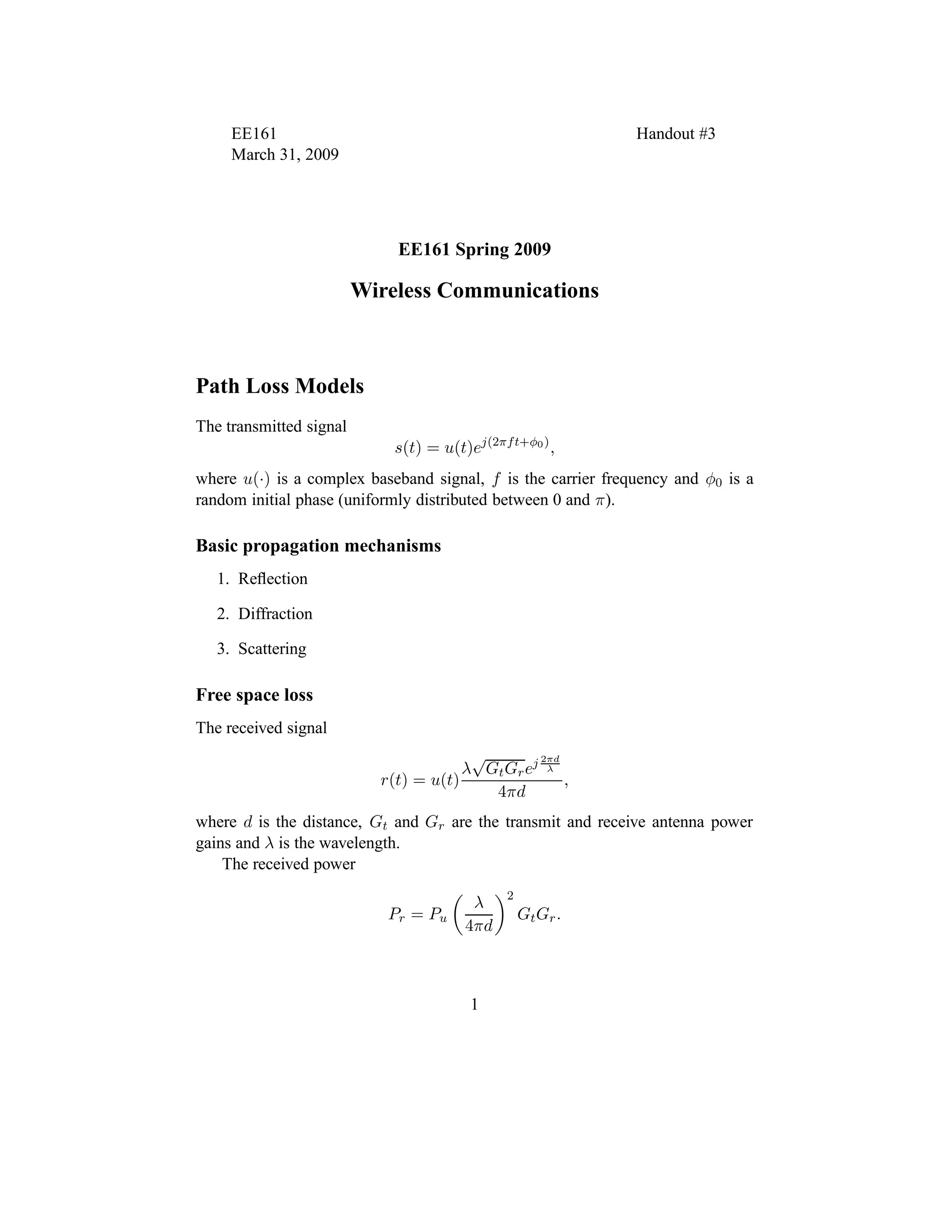
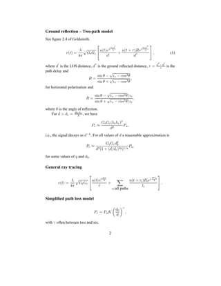
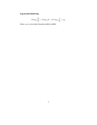
This document summarizes wireless communication path loss models. It describes the basic propagation mechanisms of reflection, diffraction, and scattering that impact signal transmission. Free space loss is defined, showing the relationship between received and transmitted power over distance. Ground reflection and the two-path model are explained, including the impact of distance on received power. General ray tracing and simplified path loss models are introduced. Finally, log-normal shadowing is summarized as modeling additional loss through a Gaussian random variable.

1. EE161 Handout #3
March 31, 2009
EE161 Spring 2009
Wireless Communications
Path Loss Models
The transmitted signal
s(t) = u(t)ej(2πft+φ0)
,
where u(·) is a complex baseband signal, f is the carrier frequency and φ0 is a
random initial phase (uniformly distributed between 0 and π).
Basic propagation mechanisms
1. Reflection
2. Diffraction
3. Scattering
Free space loss
The received signal
r(t) = u(t)
λ
√
GtGrej 2πd
λ
4πd
,
where d is the distance, Gt and Gr are the transmit and receive antenna power
gains and λ is the wavelength.
The received power
Pr = Pu
λ
4πd
2
GtGr.
1

2. Ground reflection – Two-path model
See figure 2.4 of Goldsmith.
r(t) =
λ
4π
GtGr

u(t)ej 2πd
′
λ
d′ +
u(t + τ)Rej 2πd
′′
λ
d′′

 , (1)
where d
′
is the LOS distance, d
′′
is the ground reflected distance, τ = d
′′
−d
′
c is the
path delay and
R =
sin θ −
√
ǫr − cos2θ
sin θ +
√
ǫr − cos2θ
,
for horizontal polarization and
R =
sin θ −
√
ǫr − cos2θ/ǫr
sin θ +
√
ǫr − cos2θ/ǫr
,
where θ is the angle of reflection.
For d > dc = 4hthr
λ , we have
Pr ≈
GtGr(hthr)2
d4
Pu,
i.e., the signal decays as d−4. For all values of d a reasonable approximation is
Pr ≈
GtGrd2
0
d2(1 + (d/dc)2q)1/q
Pu,
for some values of q and d0.
General ray tracing
r(t) =
λ
4π
GtGr

u(t)ej 2πl
λ
l
+
i∈all paths
u(t + τi)Riej
2πli
λ
li

 .
Simplified path loss model
Pr = PuK
d0
d
γ
,
with γ often between two and six.
2

3. Log-normal shadowing
10 log10
Pr
Pu
= 10 log10 K − 10γ log10
d
d0
+ ψdb,
where ψdb is a zero-mean Gaussian random variable.
3