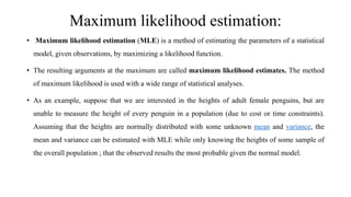
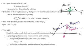
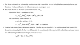
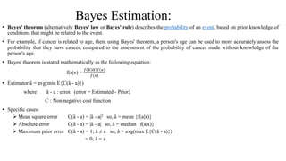
Maximum likelihood estimation finds the parameters that make the observed data most probable given a statistical model. For example, it can estimate the mean and variance of penguin heights from a sample, assuming heights are normally distributed. Bayes estimation uses Bayes' theorem and assigns costs to errors between the estimated and actual parameters. The Bayes estimate minimizes the expected cost. For a squared error cost function, the Bayes estimate is the mean of the posterior probability distribution given the data. This minimizes the mean squared error between the estimate and the actual parameter value.

1. Maximum likelihood estimation
&
Bayes Estimation
Presenting By
O.Nagamani
182041006

2. Maximum likelihood estimation:
• Maximum likelihood estimation (MLE) is a method of estimating the parameters of a statistical
model, given observations, by maximizing a likelihood function.
• The resulting arguments at the maximum are called maximum likelihood estimates. The method
of maximum likelihood is used with a wide range of statistical analyses.
• As an example, suppose that we are interested in the heights of adult female penguins, but are
unable to measure the height of every penguin in a population (due to cost or time constraints).
Assuming that the heights are normally distributed with some unknown mean and variance, the
mean and variance can be estimated with MLE while only knowing the heights of some sample of
the overall population ; that the observed results the most probable given the normal model.

3.  MLE gives the observation of x0;the,
ȃ=avg(max{f(x0; a)})
Assume that a is deterministic but unknown
 Probability of observing data x near x0 ; the fig shows the probability density function f(x;a)
then its distribution function is given by
𝑥˳−△/2
𝑥˳+△/2
𝑓 𝑥; 𝑎 𝑑𝑥 ~ 𝑓 𝑥˳; 𝑎 △ for small values of △
 MLE finds the a that gives the max probability of observing x0
it gives max 𝑓 𝑥˳; 𝑎
 Why MLE:
• Straight forward approach: Analytical or numerical optimization problem
• Asymptotic properties(numerical of measurements tends to infinity)
• MLE gives the real value (the value doesn’t give infinity)
E{ȃMLE} = a
• MLE will gives the smallest possible variance of any unbiased estimator

4. Bayes Estimation:
• Bayes' theorem (alternatively Bayes' law or Bayes' rule) describes the probability of an event, based on prior knowledge of
conditions that might be related to the event.
• For example, if cancer is related to age, then, using Bayes' theorem, a person's age can be used to more accurately assess the
probability that they have cancer, compared to the assessment of the probability of cancer made without knowledge of the
person's age.
• Bayes' theorem is stated mathematically as the following equation:
f(a|x) =
𝑓 𝑥 𝑎 𝑓 𝑎
𝑓(𝑥)
• Estimator ȃ = avg(min E{C(ȃ - a)})
where ȃ - a : error. (error = Estimated - Prior)
C : Non negative cost function
• Specific cases:
 Mean square error C(ȃ - a) = |ȃ - a|2 so, ȃ = mean {f(a|x)}
 Absolute error C(ȃ - a) = |ȃ - a| so, ȃ = median {f(a|x)}
 Maximum prior error C(ȃ - a) = 1; ȃ ≠ a so, ȃ = avg(max E{C(ȃ - a)})
= 0; ȃ = a

5. • In the Bayes detection problem we saw that the two quantities we had to specify were the set of costs Cij and the a
priori probabilities Pi . The cost matrix assigned a cost to each possible course of action. Because there were M
hypotheses and M possible decisions, there were M2 costs.
• In the estimation problem a and ci(R) are continuous variables. Thus we must assign a cost to all pairs [a, a(R)] over
the range of interest. This is a function of two variables which we denote as C(a, ȃ). In many cases of interest it is
realistic to assume that the cost depends only on the error of the estimate.
We define this error as
aϵ(R) △ ȃ(R) - a. (error = estimated - prior )
• The cost function is simply the square of the error:
C(aϵ) = aϵ
2
• This cost is commonly referred to as the squared error cost function. We see that it accentuates the effects of large
errors. The cost function is the absolute value of the error:
C(aϵ) = ‫׀‬aϵ‫׀‬

6. • First, we should like the cost function to measure user satisfaction adequately. Frequently it is difficult to assign an
analytic measure to what basically may be a subjective quality.
• Our goal is to find an estimate that minimizes the expected value of the cost. In practice, cost functions are usually some
compromise between these two objectives. Fortunately, in many problems of interest the same estimate will be optimum
for a large class of cost functions.
• Corresponding to the a priori probabilities in the detection problem, we have an a priori probability density pa(A) in the
random parameter estima- tion problem. In all of our discussions we assume that pa(A) is known.
• If pa(A) is not known, a procedure analogous to the minimax test may be used. Once we have specified the cost function
and the a priori probability, we may write an expression for the risk:
R △ E{C[a, ȃ(R)]} = −∞
∞
𝑑𝐴 −∞
∞
C[A, ȃ(R)]pa,R(A,R) dR
• The expectation is over the random variable a and the observed variables r. For costs that are functions of one variable
only becomes
R= −∞
∞
𝑑𝐴 −∞
∞
C[A, ȃ(R)]pa,R(A,R) dR

7. • The Bayes estimate is the estimate that minimizes the risk. It is straight- forward to find the Bayes estimates for the cost
functions. For the cost function the risk corresponds to mean-square error.
• We denote the risk for the mean-square error criterion as Rms
Substituting above 2 equations; we have
Rms = −∞
∞
𝑑𝐴 −∞
∞
dR[A − ȃ(R)2
pa,R(A,R) dR
The joint density can be rewritten as
pa,R(A, R) = pr(R)pa‫׀‬R (A/R).
Rms = −∞
∞
𝑑𝑅 𝑝 𝑟 𝑅 −∞
∞
dA[A − ȃ(R)2
pa,/R(A/R) dR
• Now the inner integral and pr(R) are non negative. Therefore we can minimize Rms by minimizing the inner integral. We
denote this estimate ȃms(R). To find it we differentiate the inner integral with respect to ȃ(R) and set the result equal to zero
and and observing that the second integral equals 1, we have
ȃms(R) = −∞
∞
𝑑𝐴 𝐴𝑝 𝑎/𝑟(A/R)

8. • This is a unique minimum, for the second derivative equals two. The term on the right side is familiar as the mean of the
a posteriori density (or the conditional mean).
• we see that if ȃ(R) is the conditional mean the inner integral is just the a posteriori variance (or the conditional variance).
Therefore the minimum value of Rms is just the average of the conditional variance over all observations R.