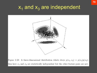
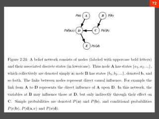
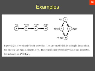
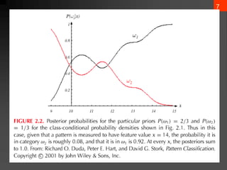
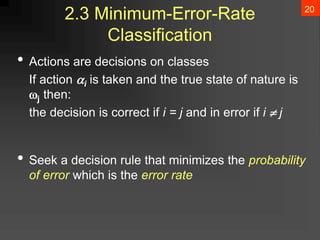
The document discusses Bayesian decision theory, focusing on its application in machine learning for classification tasks. It covers concepts such as minimum-error-rate classification, decision rules based on posterior probabilities, and the use of loss functions to guide decision-making under uncertainty. Additionally, it explores the mathematical formulations for discriminant functions and the properties of normal density in relation to classification problems.

1. Machine Learning

2. Bayesian Decision Theory
1. Introduction – Bayesian Decision Theory
• Pure statistics, probabilities known, optimal decision
2. Bayesian Decision Theory–Continuous Features
3. Minimum-Error-Rate Classification
4. Classifiers, Discriminant Functions, Decision Surfaces
5. The Normal Density
6. Discriminant Functions for the Normal Density

3. 2
1. Introduction
• The sea bass/salmon example
• State of nature, prior
• State of nature is a random variable
• The catch of salmon and sea bass is equiprobable
• P(1) = P(2) (uniform priors)
• P(1) + P( 2) = 1 (exclusivity and exhaustivity)

4. 3
• Decision rule with only the prior information
• Decide 1 if P(1) > P(2) otherwise decide 2
• Use of the class –conditional information
• p(x | 1) and p(x | 2) describe the difference in
lightness between populations of sea and salmon

5. 4

6. Bayes Formula
• Suppose we know the prior probabilities P(j) and
the conditional densities p(x | j) for j = 1, 2.
• Lightness of a fish has value x
• Joint probability density of finding a pattern that is
in category j and has feature value x:
• p(j , x) = P(j | x) p(x) = p(x | j) P(j)
5

7. 6
• Posterior, likelihood, evidence
• P(j | x) = P(x | j) P (j) / P(x) (Bayes Rule)
• Where in case of two categories
• Posterior = (Likelihood. Prior) / Evidence




2
j
1
j
j
j )
(
P
)
|
x
(
P
)
x
(
P 


8. 7

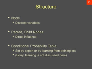
9. 8
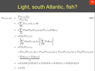
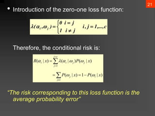
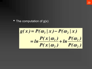
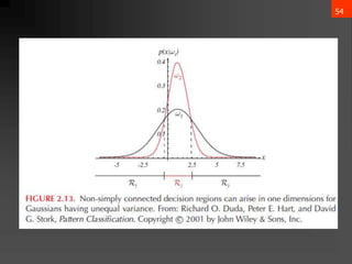
• Decision given the posterior probabilities
X is an observation for which:
if P(1 | x) > P(2 | x) True state of nature = 1
if P(1 | x) < P(2 | x) True state of nature = 2
This rule minimizes average probability of error:
𝑃 ⅇ𝑟𝑟𝑜𝑟 =
−∞
∞
𝑝 ⅇ𝑟𝑟𝑜𝑟, 𝑥 ⅆ𝑥 =
−∞
∞
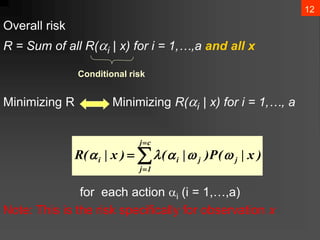
𝑝 ⅇ𝑟𝑟𝑜𝑟 𝑥 𝑝 𝑥 𝑑𝑥
p ⅇ𝑟𝑟𝑜𝑟 𝑥 = min[P(1 | x), P(2 | x) ]
Decide 1 if P(x | 1) P (1) > P(x | 2) P (2)

10. 9
2. Bayesian Decision Theory –
Continuous Features
• Generalization of the preceding ideas
1. Use of more than one feature, vector X
2. Use more than two states of nature, c classes
3. Allowing actions other than deciding the state of nature
4. Introduce a loss of function which is more general than
the probability of error

11. 10
• Allowing actions other than classification primarily
allows the possibility of rejection
• Rejection in the sense of abstention
• Don’t make a decision if the alternatives are too close
• This must be tempered by the cost of indecision
• The loss function states how costly each action
taken is

12. 11
Let {1, 2,…, c} be the set of c states of nature
(or “categories”)
Let {1, 2,…, a} be the set of possible actions
Let (i | j) be the loss incurred for taking
action i when the state of nature is j

13. 12
Overall risk
R = Sum of all R(i | x) for i = 1,…,a and all x
Minimizing R Minimizing R(i | x) for i = 1,…, a
for each action i (i = 1,…,a)
Note: This is the risk specifically for observation x
Conditional risk




c
j
1
j
j
j
i
i )
x
|
(
P
)
|
(
)
x
|
(
R 





14. 13
Select the action i for which R(i | x) is minimum
R is minimum and R in this case is called the
Bayes risk = best performance that can be achieved!

15. 14
• Two-category classification
1 : deciding 1
2 : deciding 2
ij = (i | j)
loss incurred for deciding i when the true state of nature is j
Conditional risk:
R(1 | x) = 11P(1 | x) + 12P(2 | x)
R(2 | x) = 21P(1 | x) + 22P(2 | x)

16. 15
Our rule is the following:
if R(1 | x) < R(2 | x)
action 1: “decide 1” is taken
Substituting the def. of R() we have :
decide 1 if:
11 P(1 | x) + 12P(2 | x) <
21 P(1 | x) + 22P(2 | x)
and decide 2 otherwise

17. 16
We can rewrite
11 P(1 | x) + 12P(2 | x) <
21 P(1 | x) + 22P(2 | x)
As
(21- 11) P(1 | x) > (12- 22) P(2 | x)

18. 17
Finally, we can rewrite
(21- 11) P(1 | x) >
(12- 22) P(2 | x)
using Bayes formula and posterior probabilities to
get:
decide 1 if:
(21- 11) P(x | 1) P(1) >
(12- 22) P(x | 2) P(2)
and decide 2 otherwise

19. 18
If 21 > 11 then we can express our rule as a
Likelihood ratio:
The preceding rule is equivalent to the following rule:
Then take action 1 (decide 1)
Otherwise take action 2 (decide 2)
)
(
P
)
(
P
.
)
|
x
(
P
)
|
x
(
P
if
1
2
11
21
22
12
2
1












20. 19
Optimal decision property
“If the likelihood ratio exceeds a threshold value
independent of the input pattern x, we can take
optimal actions”

21. 20
2.3 Minimum-Error-Rate
Classification
• Actions are decisions on classes
If action i is taken and the true state of nature is
j then:
the decision is correct if i = j and in error if i  j
• Seek a decision rule that minimizes the probability
of error which is the error rate

22. 21
• Introduction of the zero-one loss function:
Therefore, the conditional risk is:
“The risk corresponding to this loss function is the
average probability error”
c
,...,
1
j
,
i
j
i
1
j
i
0
)
,
( j
i 


















i
j
i
j
c
j
j
j
j
i
i
x
P
x
P
x
P
x
R
)
|
(
1
)
|
(
)
|
(
)
|
(
)
|
(
1








23. 22
• Minimize the risk requires maximize P(i | x)
(since R(i | x) = 1 – P(i | x))
• For Minimum error rate
• Decide i if P (i | x) > P(j | x) j  i

24. 23
• Regions of decision and zero-one loss function,
therefore:
• If  is the zero-one loss function which means:
b
1
2
a
1
2
)
(
P
)
(
P
2
then
0
1
2
0
if
)
(
P
)
(
P
then
0
1
1
0



































 














)
|
x
(
P
)
|
x
(
P
:
if
decide
then
)
(
P
)
(
P
.
Let
2
1
1
1
2
11
21
22
12

25. 24

26. 25
4. Classifiers, Discriminant Functions,
and Decision Surfaces
• The multi-category case
• Set of discriminant functions gi(x), i = 1,…, c
• The classifier assigns a feature vector x to class i
if:
gi(x) > gj(x) j  i

27. 26
• Discriminant function
gi(x) = P(i | x)
(max. discrimination corresponds to max.
posterior!)
gi(x)  P(x | i) P(i)
gi(x) = ln P(x | i) + ln P(i)
(ln: natural logarithm!)

28. 27

29. 28
• Feature space divided into c decision regions
if gi(x) > gj(x) j  i then x is in Ri
(Ri means assign x to i)
• The two-category case
• A classifier is a “dichotomizer” that has two discriminant
functions g1 and g2
Let g(x)  g1(x) – g2(x)
Decide 1 if g(x) > 0 ; Otherwise decide 2

30. 29
• The computation of g(x)
)
(
P
)
(
P
ln
)
|
x
(
P
)
|
x
(
P
ln
)
x
|
(
P
)
x
|
(
P
)
x
(
g
2
1
2
1
2
1











31. 30

32. 31
5. The Normal Density
• Univariate density
• Density which is analytically tractable
• Continuous density
• A lot of processes are asymptotically Gaussian
• Handwritten characters, speech sounds are ideal or prototype
corrupted by random process (central limit theorem)
Where:
 = mean (or expected value) of x
2 = expected squared standard deviation or variance
,
x
2
1
exp
2
1
)
x
(
P
2













 







33. 32

34. 33
• Multivariate normal density p(x) ~ N(, )
• Multivariate normal density in d dimensions is:
where:
x = (x1, x2, …, xd)t (t stands for the transpose vector form)
 = (1, 2, …, d)t mean vector
 = d*d covariance matrix
|| and -1 are determinant and inverse respectively









 
)
x
(
)
x
(
2
1
exp
)
2
(
1
)
x
(
P 1
t
2
/
1
2
/
d




 

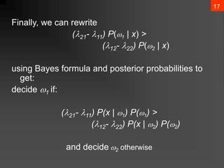
35. 34
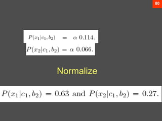
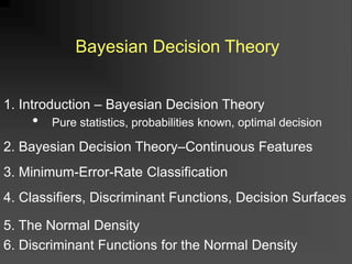
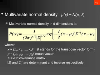
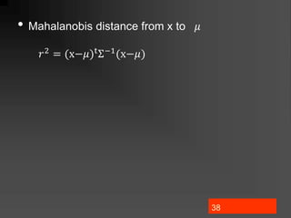
𝜇 = 𝜀[x] = x𝑝(x)𝑑x
∑ = 𝜀[(x−𝜇)(x−𝜇)t] = (x−𝜇)(x−𝜇)t𝑝(x)𝑑x
𝜇𝑖 = 𝜀[𝑥𝑖]
𝜎𝑖𝑗 = 𝜀[(𝑥𝑖 − 𝜇𝑖)(𝑥𝑗 − 𝜇𝑗)]

36. • Always symmetric
• Always positive semi-definite, but for our purposes
 is positive definite
• determinant is positive
•  invertible
• Eigenvalues real and positive,
Properties of the Normal Density
Covariance Matrix 

37. 36
• Linear combinations of normally distributed random
variables are normally distributed
if
then
• Whitening transform:
:The orthonormal eigenvectors of
:The diagonal matrix of the eigenvalues
𝑝(x)~𝑁(𝜇, ∑), 𝐴: 𝑑 × 𝑘, y = 𝐴𝑡x
𝑝(y)~𝑁(At𝜇, AtΣA)
𝐴𝑤 = ΦΛ−1/2
Φ Σ
Λ

38. 37


39. 38
• Mahalanobis distance from x to 𝜇
𝑟2 = (x−𝜇)tΣ−1(x−𝜇)

40. 39


41. 40
• Entropy
• Measure the fundamental uncertainty in the
values of points selected randomly
• Measured in nats, bit,
• Normal distribution has max entropy of all
distributions having a given mean and variance
𝐻(𝑝(𝑥)) = − 𝑝(𝑥) ln 𝑝 (𝑥)𝑑𝑥

42. 41
6. Discriminant Functions for the
Normal Density
• We saw that the minimum error-rate classification
can be achieved by the discriminant function
gi(x) = ln P(x | i) + ln P(i)
• Case of multivariate normal p(x) ~ N(, )
)
(
P
ln
ln
2
1
2
ln
2
d
)
x
(
)
x
(
2
1
)
x
(
g i
i
1
i
i
t
i
i 



 





 


43. 42
Case i = 2I (I stands for the identity matrix)
• What does “i = 2I” say about the
dimensions?
• What about the variance of each dimension?
norm
Euclidean
the
denotes
where
)
(
ln
2
)
(
:
o
simplify t
can
we
Thus
)
(
ln
ln
2
1
2
ln
2
)
(
)
(
2
1
)
(
in
of
t
independen
are
ln
(d/2)
and
both
:
Note
2
2
1
i
















i
i
i
i
i
i
i
t
i
i
P
x
g
P
d
x
x
x
g
i










44. 43
1.Case i = 2 I (I stands for the identity matrix)
We can further simplify by recognizing that the quadratic term xtx implicit
in the Euclidean norm is the same for all i.
)
category!
th
the
for
threshold
the
called
is
(
)
(
P
ln
2
1
w
;
w
:
where
function)
nt
discrimina
(linear
w
x
w
)
x
(
g
0
i
i
i
t
i
2
0
i
2
i
i
0
i
t
i
i
i














45. 44
• A classifier that uses linear discriminant functions is
called “a linear machine”
• The decision surfaces for a linear machine are
pieces of hyperplanes defined by:
gi(x) = gj(x)
The equation can be written as:
wt(x-x0)=0
• If equal priors for all classes, this reduces to the
minimum-distance classifier where an unknown is
assigned to the class of the nearest mean

46. 45
• The hyperplane separating Ri and Rj
always orthogonal to the line linking the means!
)
(
)
(
P
)
(
P
ln
)
(
2
1
x j
i
j
i
2
j
i
2
j
i
0 







 




)
(
2
1
x
then
)
(
P
)
(
P
if j
i
0
j
i 


 



47. 46

48. 47

49. 48

50. • 2. Case i =  (covariance of all classes are
identical but arbitrary!)
The quadratic form (𝑥 − 𝜇𝑖)𝑡 ∑𝑖
−1
(𝑥 − 𝜇𝑖) results in a sum involving a
quadratic term xt -1x which is independent of i.
After this term is dropped, the resulting discriminant function is again linear
49
Notⅇ: both Σi anⅆ (ⅆ/2) ln𝜋 arⅇ inⅆⅇpⅇnⅆⅇnt of 𝑖 in
𝑔𝑖(𝑥) = −
1
2
(𝑥 − 𝜇𝑖)𝑡
𝑖
−1
(𝑥 − 𝜇𝑖) −
𝑑
2
ln 2 𝜋 −
1
2
ln Σ𝑖 + ln 𝑃 (𝜔𝑖)
Thus wⅇ can simplify to:
𝑔𝑖(𝑥) = −
1
2
(𝑥 − 𝜇𝑖)𝑡
𝑖
−1
(𝑥 − 𝜇𝑖) + ln 𝑃 (𝜔𝑖)
whⅇrⅇ (𝑥 − 𝜇𝑖)𝑡
𝑖
−1
(𝑥 − 𝜇𝑖) ⅆⅇnotⅇs thⅇ Mahalanobis ⅆistancⅇ

51. 50
𝑔𝑖(𝑥) = 𝑤𝑖
𝑡
𝑥 + 𝑤𝑖0 (linⅇar ⅆiscriminant function)
whⅇrⅇ:
𝑤𝑖 = −1𝜇𝑖; 𝑤𝑖0 = −
1
2
𝜇𝑖
𝑡
−1𝜇𝑖 + ln 𝑃 (𝜔𝑖)
(𝜔𝑖0 is callⅇⅆ thⅇ thrⅇsholⅆ for thⅇ ith catⅇgory!)
The resulting decision boundaries are again hyperplanes.
If Ri and Rj are contiguous, the boundary between them has the
equation:
wt(x-x0)=0
W = −1(𝜇𝑖 - 𝜇j)

52. 51
2. Case i =  (covariance of all classes are identical
but arbitrary!)
• Hyperplane separating Ri and Rj
(the hyperplane separating Ri and Rj is generally not
orthogonal to the line between the means!)
If priors are equal, 𝑥0 is half way between the means.
𝑥0 =
1
2
(𝜇𝑖 + 𝜇𝑗) −
ln 𝑃(𝜔𝑖)/𝑃(𝜔𝑗)
(𝜇𝑖 − 𝜇𝑗)𝑡Σ−1(𝜇𝑖 − 𝜇𝑗)
. (𝜇𝑖 − 𝜇𝑗)

53. 52

54. 53

55. 54

56. 55
3. Case i = arbitrary
• The covariance matrices are different for each category
(Hyperquadrics which are: hyperplanes, pairs of hyperplanes,
hyperspheres, hyperellipsoids, hyperparaboloids,
hyperhyperboloids)
𝑔𝑖 𝑥 = 𝑥𝑡𝑊𝑖𝑥 + 𝑤𝑖
𝑡
𝑥 + 𝑤𝑖0
𝑤ℎ𝑒𝑟𝑒:
Wi = −
1
2
Σ𝑖
−1
wi = Σ𝑖
−1
𝜇𝑖
w𝑖0 = −
1
2
𝜇𝑖
𝑡
Σ𝑖
−1
𝜇𝑖 −
1
2
ln Σ𝑖 + ln 𝑃 (𝜔𝑖)
)
(
P
ln
ln
2
1
2
1
w
w
2
1
W
:
where
w
x
w
x
W
x
)
x
(
g
i
i
i
1
i
t
i
0
i
i
1
i
i
1
i
i
0
i
t
i
i
t
i






















57. 56

58. 57

59. 58

60. 59

61. 60

62. 61

63. Assume we have following data

64. 63
Bayes Decision Theory – Discrete
Features
• Components of x are binary or integer valued, x can take
only one of m discrete values
v1, v2, …, vm
 concerned with probabilities rather than probability
densities in Bayes Formula:




c
j
j
j
j
j
j
P
P
P
P
P
P
P
1
)
(
)
|
(
)
(
where
)
(
)
(
)
|
(
)
|
(





x
x
x
x
x

65. 64
Bayes Decision Theory – Discrete
Features
• Conditional risk is defined as before: R(|x)
• Approach is still to minimize risk:
)
|
(
min
arg
*
x
i
i
R 
 

66. 65
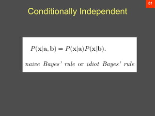
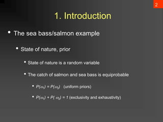
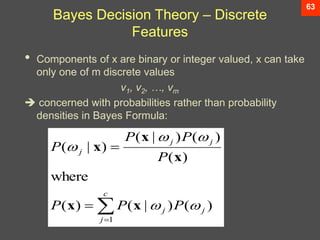
Bayes Decision Theory – Discrete
Features
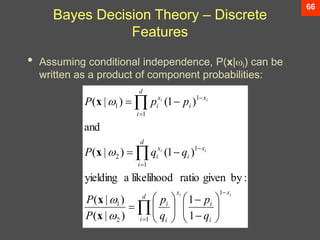
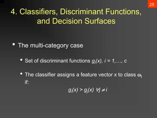
• Case of independent binary features in 2
category problem
Let x = [x1, x2, …, xd ]t where each xi is either 0
or 1, with probabilities:
pi = P(xi = 1 | 1)
qi = P(xi = 1 | 2)

67. 66
Bayes Decision Theory – Discrete
Features
• Assuming conditional independence, P(x|i) can be
written as a product of component probabilities:
































d
i
x
i
i
x
i
i
d
i
x
i
x
i
d
i
x
i
x
i
i
i
i
i
i
i
q
p
q
p
P
P
q
q
P
p
p
P
1
1
2
1
1
1
2
1
1
1
1
1
)
|
(
)
|
(
:
by
given
ratio
likelihood
a
yielding
)
1
(
)
|
(
and
)
1
(
)
|
(




x
x
x
x

68. 67
Bayes Decision Theory – Discrete
Features
• Taking our likelihood ratio
)
(
)
(
ln
1
1
ln
)
1
(
ln
)
(
:
yields
)
(
)
(
ln
)
|
(
)
|
(
ln
)
(
31
Eq.
into
it
plugging
and
1
1
)
|
(
)
|
(
2
1
1
2
1
2
1
1
1
2
1








p
p
q
p
x
q
p
x
g
p
p
p
p
g
q
p
q
p
P
P
d
i i
i
i
i
i
i
d
i
x
i
i
x
i
i
i
i






































x
x
x
x
x
x

69. 68
• The discriminant function in this case is:
0
g(x)
if
and
0
g(x)
if
decide
)
(
P
)
(
P
ln
q
1
p
1
ln
w
:
and
d
,...,
1
i
)
p
1
(
q
)
q
1
(
p
ln
w
:
where
w
x
w
)
x
(
g
2
1
2
1
d
1
i i
i
0
i
i
i
i
i
0
i
d
1
i
i





















70. 69
Bayesian Belief Network
• Features
• Causal relationships
• Statistically independent
• Bayesian belief nets
• Causal networks
• Belief nets

71. 70
x1 and x3 are independent

72. 71
Structure
• Node
• Discrete variables
• Parent, Child Nodes
• Direct influence
• Conditional Probability Table
• Set by expert or by learning from training set
• (Sorry, learning is not discussed here)

73. 72

74. 73
Examples

75. 74

76. 75

77. 76
Evidence e

78. 77
Ex. 4. Belief Network for Fish
A B
X
C D
P(a)
P(b)
P(c|x)
P(d|x)
P(x|a,b)
b1=north Atlantic, 0.6
b2=south Atlantic, 0.4
a1=winter, 0.25
a2=spring, 0.25
a3=summer,0.25
a4=autumn, 0.25
x1=salmon
x2=sea bass
d1=wide, d2=thin
x1 0.3, 0.7
x2 0.6, 0.4
c1=light,c2=medium, c3=dark
x1 0.6, 0.2, 0.2
x2 0.2, 0.3, 0.5
x1 x2
a1b1 0.5 0.5
a1b2 0.7 0.3
a2b1 0.6 0.4
a2b2 0.8 0.2
a3b1 0.4 0.6
a3b2 0.1 0.9
a4b1 0.2 0.8
a4b2 0.3 0.7

79. 78
Belief Network for Fish
• Fish was caught in the summer in the north
Atlantic and is a sea bass that is dark and thin
• P(a3,b1,x2,c3,d2)
= P(a3)P(b1)P(x2|a3,b1)P(c3|x2)P(d2|x2)
=0.25*0.6*0.6*0.5*0.4
=0.018

80. Pattern Classification, Chapter 2 (Part 3)
79
Light, south Atlantic, fish?

81. 80
Normalize

82. 81
Conditionally Independent

83. 82
Medical Application
• Medical diagnosis
• Uppermost nodes: biological agent
• (virus or bacteria)
• Intermediate nodes: diseases
• (flu or emphysema)
• Lowermost nodes: symptoms
• (high temperature or coughing)
• Finds the most likely disease or cause
• By entering measured values