This document summarizes key points from Lecture 2 of the Introduction to Programming in MATLAB course. It discusses user-defined functions, including function declarations and overloading functions. Flow control statements like if/else and for loops are explained. Various plotting functions and options are covered, such as line, image, surface, and 3D plots. Advanced plotting exercises demonstrate modifying a plotting function to include conditionals and subplotting multiple axes. Specialized plotting functions like polar, bar, and quiver are also mentioned.

1. 6.094
Introduction to programming in MATLAB
Lecture 2: Visualization and Programming
Danilo Šćepanović
IAP 2010

2. Homework 1 Recap
•
•
•
•
How long did it take to do required problems?
Did anyone do optional problems?
Was level of guidance appropriate?
Unanswered Questions?
• Some things that came up:
• Use of semicolon – never required if one command per line.
You can also put multiple commands on one line; in this
case a semicolon is necessary to separate commands:
» x=1:10; y=(x-5).^2; plot(x,y);
• Assignment using indices – remember that you can index
into matrices to either look up values or to assign value:
» x=rand(50,1); inds=find(x<0.1); y=x(inds);
x(inds)=-x(inds); x(inds)=3;

3. Outline
(1)
(2)
(3)
(4)
(5)
Functions
Flow Control
Line Plots
Image/Surface Plots
Vectorization

4. User-defined Functions
• Functions look exactly like scripts, but for ONE difference
Functions must have a function declaration
Help file
Function declaration
Outputs
Inputs
Courtesy of The MathWorks, Inc. Used with permission.

5. User-defined Functions
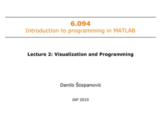
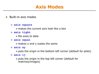
• Some comments about the function declaration
Inputs must be specified
function [x, y, z] = funName(in1, in2)
Function name should
match MATLAB file
name
If more than one output,
must be in brackets
Must have the reserved
word: function
• No need for return: MATLAB 'returns' the variables whose
names match those in the function declaration
• Variable scope: Any variables created within the function
but not returned disappear after the function stops running

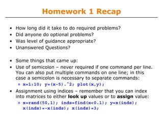
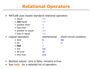
6. Functions: overloading
• We're familiar with
» zeros
» size
» length
» sum
• Look at the help file for size by typing
» help size
• The help file describes several ways to invoke the function
D = SIZE(X)
[M,N] = SIZE(X)
[M1,M2,M3,...,MN] = SIZE(X)
M = SIZE(X,DIM)

7. Functions: overloading
• MATLAB functions are generally overloaded
Can take a variable number of inputs
Can return a variable number of outputs
• What would the following commands return:
» a=zeros(2,4,8); %n-dimensional matrices are OK
» D=size(a)
» [m,n]=size(a)
» [x,y,z]=size(a)
» m2=size(a,2)
• You can overload your own functions by having variable
input and output arguments (see varargin, nargin,
varargout, nargout)

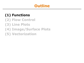
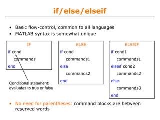
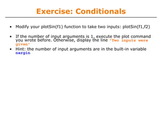
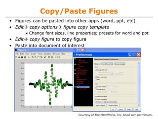
8. Functions: Excercise
• Write a function with the following declaration:
function plotSin(f1)
• In the function, plot a sin wave with frequency f1, on the
range [0,2π]: sin ( f1 x )
• To get good sampling, use 16 points per period.
1
0.8
0.6
0.4
0.2
0
-0.2
-0.4
-0.6
-0.8
-1
0
1
2
3
4
5
6
7

9. Functions: Excercise
• Write a function with the following declaration:
function plotSin(f1)
• In the function, plot a sin wave with frequency f1, on the
range [0,2π]: sin ( f1 x )
• To get good sampling, use 16 points per period.
• In an MATLAB file saved as plotSin.m, write the following:
» function plotSin(f1)
x=linspace(0,2*pi,f1*16+1);
figure
plot(x,sin(f1*x))

10. Outline
(1)
(2)
(3)
(4)
(5)
Functions
Flow Control
Line Plots
Image/Surface Plots
Vectorization

11. Relational Operators
• MATLAB uses mostly standard relational operators
equal
not equal
greater than
less than
greater or equal
less or equal
• Logical operators
And
Or
Not
Xor
All true
Any true
==
~=
>
<
>=
<=
elementwise
short-circuit (scalars)
&
|
~
xor
all
any
&&
||
• Boolean values: zero is false, nonzero is true
• See help . for a detailed list of operators

12. if/else/elseif
• Basic flow-control, common to all languages
• MATLAB syntax is somewhat unique
IF
if cond
commands
end
ELSE
if cond
commands1
else
commands2
Conditional statement:
evaluates to true or false
end
ELSEIF
if cond1
commands1
elseif cond2
commands2
else
commands3
end
• No need for parentheses: command blocks are between
reserved words

13. for
• for loops: use for a known number of iterations
• MATLAB syntax:
Loop variable
for n=1:100
commands
end
Command block
• The loop variable
Is defined as a vector
Is a scalar within the command block
Does not have to have consecutive values (but it's usually
cleaner if they're consecutive)
• The command block
Anything between the for line and the end

14. while
• The while is like a more general for loop:
Don't need to know number of iterations
WHILE
while cond
commands
end
• The command block will execute while the conditional
expression is true
• Beware of infinite loops!

15. Exercise: Conditionals
• Modify your plotSin(f1) function to take two inputs: plotSin(f1,f2)
• If the number of input arguments is 1, execute the plot command
you wrote before. Otherwise, display the line 'Two inputs were
given'
• Hint: the number of input arguments are in the built-in variable
nargin

16. Exercise: Conditionals
• Modify your plotSin(f1) function to take two inputs:
plotSin(f1,f2)
• If the number of input arguments is 1, execute the plot command
you wrote before. Otherwise, display the line 'Two inputs were
given'
• Hint: the number of input arguments are in the built-in variable
nargin
» function plotSin(f1,f2)
x=linspace(0,2*pi,f1*16+1);
figure
if nargin == 1
plot(x,sin(f1*x));
elseif nargin == 2
disp('Two inputs were given');
end

17. Outline
(1)
(2)
(3)
(4)
(5)
Functions
Flow Control
Line Plots
Image/Surface Plots
Vectorization

18. Plot Options
• Can change the line color, marker style, and line style by
adding a string argument
» plot(x,y,’k.-’);
color
marker
line-style
• Can plot without connecting the dots by omitting line style
argument
» plot(x,y,’.’)
• Look at help plot for a full list of colors, markers, and
linestyles

19. Playing with the Plot
to select lines
and delete or
change
properties
to zoom in/out
to slide the plot
around
to see all plot
tools at once
Courtesy of The MathWorks, Inc. Used with permission.

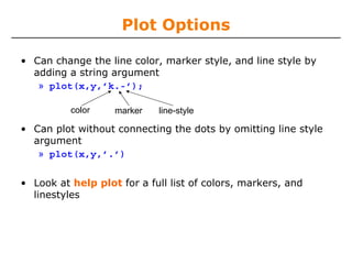
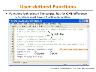
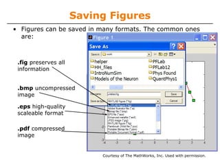
20. Line and Marker Options
• Everything on a line can be customized
» plot(x,y,'--s','LineWidth',2,...
'Color', [1 0 0], ...
'MarkerEdgeColor','k',...
'MarkerFaceColor','g',...
'MarkerSize',10)
You can set colors by using
a vector of [R G B] values
or a predefined color
character like 'g', 'k', etc.
0.8
0.6
0.4
0.2
0
• See doc line_props for a full list of-0.2
properties that can be specified
-0.4
-0.6
-0.8
-4
-3
-2
-1
0
1
2
3
4

21. Cartesian Plots
• We have already seen the plot function
» x=-pi:pi/100:pi;
» y=cos(4*x).*sin(10*x).*exp(-abs(x));
» plot(x,y,'k-');
• The same syntax applies for semilog and loglog plots
» semilogx(x,y,'k');
» semilogy(y,'r.-');
» loglog(x,y);
50
10
40
10
30
10
• For example:
» x=0:100;
» semilogy(x,exp(x),'k.-');
20
10
10
10
0
10
0
10
20
30
40
50
60
70
80
90
100

22. 3D Line Plots
• We can plot in 3 dimensions just as easily as in 2
» time=0:0.001:4*pi;
» x=sin(time);
» y=cos(time);
» z=time;
» plot3(x,y,z,'k','LineWidth',2);
» zlabel('Time');
10
• Use tools on figure to rotate it
• Can set limits on all 3 axes
» xlim, ylim, zlim
5
0
-5
-10
1
0.5
1
0.5
0
0
-0.5
-0.5
-1
-1

23. Axis Modes
• Built-in axis modes
» axis square
makes the current axis look like a box
» axis tight
fits axes to data
» axis equal
makes x and y scales the same
» axis xy
puts the origin in the bottom left corner (default for plots)
» axis ij
puts the origin in the top left corner (default for
matrices/images)

24. Multiple Plots in one Figure
• To have multiple axes in one figure
» subplot(2,3,1)
makes a figure with 2 rows and three columns of axes, and
activates the first axis for plotting
each axis can have labels, a legend, and a title
» subplot(2,3,4:6)
activating a range of axes fuses them into one
• To close existing figures
» close([1 3])
closes figures 1 and 3
» close all
closes all figures (useful in scripts/functions)

25. Copy/Paste Figures
• Figures can be pasted into other apps (word, ppt, etc)
• Edit copy options figure copy template
Change font sizes, line properties; presets for word and ppt
• Edit copy figure to copy figure
• Paste into document of interest
Courtesy of The MathWorks, Inc. Used with permission.

26. Saving Figures
• Figures can be saved in many formats. The common ones
are:
.fig preserves all
information
.bmp uncompressed
image
.eps high-quality
scaleable format
.pdf compressed
image
Courtesy of The MathWorks, Inc. Used with permission.

27. Advanced Plotting: Exercise
• Modify the plot command in your plotSin function to use
squares as markers and a dashed red line of thickness 2
as the line. Set the marker face color to be black
(properties are LineWidth, MarkerFaceColor)
• If there are 2 inputs, open a new figure with 2 axes, one on
top of the other (not side by side), and activate the top one
(subplot)
plotSin(6)
plotSin(1,2)
1
1
0.8
0.8
0.6
0.6
0.4
0.4
0.2
0.2
0
0
-0.2
-0.4
-0.6
-0.8
-1
0
1
2
3
4
5
6
7
0
0.1
0.2
0.3
0.4
0.5
0.6
0.7
0.8
0.9
1

28. Advanced Plotting: Exercise
• Modify the plot command in your plotSin function to use
squares as markers and a dashed red line of thickness 2
as the line. Set the marker face color to be black
(properties are LineWidth, MarkerFaceColor)
• If there are 2 inputs, open a new figure with 2 axes, one on
top of the other (not side by side), and activate the top one
(subplot)
» if nargin == 1
plot(x,sin(f1*x),'rs--',...
'LineWidth',2,'MarkerFaceColor','k');
elseif nargin == 2
subplot(2,1,1);
end

29. Outline
(1)
(2)
(3)
(4)
(5)
Functions
Flow Control
Line Plots
Image/Surface Plots
Vectorization

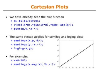
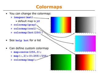
30. Visualizing matrices
• Any matrix can be visualized as an image
» mat=reshape(1:10000,100,100);
» imagesc(mat);
» colorbar
• imagesc automatically scales the values to span the entire
colormap
• Can set limits for the color axis (analogous to xlim, ylim)
» caxis([3000 7000])

31. Colormaps
• You can change the colormap:
» imagesc(mat)
default map is jet
» colormap(gray)
» colormap(cool)
» colormap(hot(256))
• See help hot for a list
• Can define custom colormap
» map=zeros(256,3);
» map(:,2)=(0:255)/255;
» colormap(map);

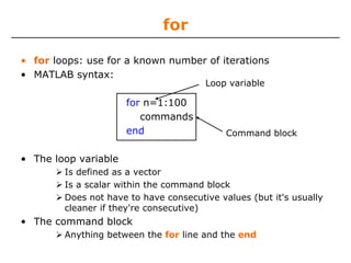
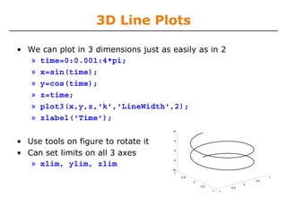
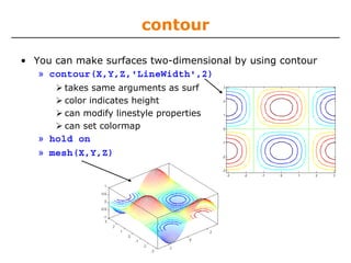
32. Surface Plots
• It is more common to visualize surfaces in 3D
• Example:
f ( x, y ) = sin ( x ) cos ( y )
x ∈ [ −π ,π ] ; y ∈ [ −π ,π ]
• surf puts vertices at specified points in space x,y,z, and
connects all the vertices to make a surface
• The vertices can be denoted by matrices X,Y,Z
3
• How can we make these matrices
loop (DUMB)
built-in function: meshgrid
2
4
3
2
6
2
1
8
4
2
10
0
6
1
12
8
-1
14
10
0
16
12
-2
18
-1
14
20
16
-3
2
-2
18
20
-3
2
4
6
8
10
12
14
16
18
20
4
6
8
10
12
14
16
18
20

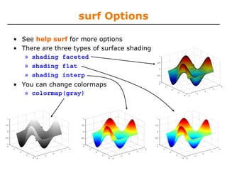
33. surf
• Make the x and y vectors
» x=-pi:0.1:pi;
» y=-pi:0.1:pi;
• Use meshgrid to make matrices (this is the same as loop)
» [X,Y]=meshgrid(x,y);
• To get function values,
evaluate the matrices
» Z =sin(X).*cos(Y);
• Plot the surface
» surf(X,Y,Z)
» surf(x,y,Z);

34. surf Options
• See help surf for more options
• There are three types of surface shading
» shading faceted
» shading flat
» shading interp
• You can change colormaps
» colormap(gray)

35. contour
• You can make surfaces two-dimensional by using contour
» contour(X,Y,Z,'LineWidth',2)
takes same arguments as surf
color indicates height
can modify linestyle properties
can set colormap
» hold on
» mesh(X,Y,Z)

36. Exercise: 3-D Plots
• Modify plotSin to do the following:
• If two inputs are given, evaluate the following function:
Z = sin ( f1 x ) + sin ( f 2 y )
• y should be just like x, but using f2. (use meshgrid to get
the X and Y matrices)
• In the top axis of your subplot, display an image of the Z
matrix. Display the colorbar and use a hot colormap. Set
the axis to xy (imagesc, colormap, colorbar, axis)
• In the bottom axis of the subplot, plot the 3-D surface of Z
(surf)

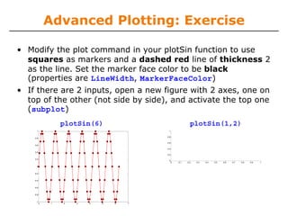
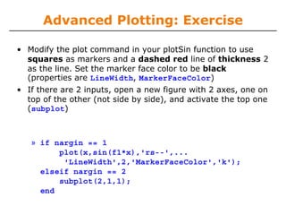
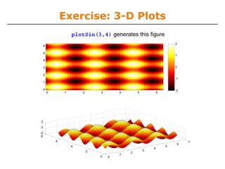
37. Exercise: 3-D Plots
» function plotSin(f1,f2)
x=linspace(0,2*pi,round(16*f1)+1);
figure
if nargin == 1
plot(x,sin(f1*x),'rs--',...
'LineWidth',2,'MarkerFaceColor','k');
elseif nargin == 2
y=linspace(0,2*pi,round(16*f2)+1);
[X,Y]=meshgrid(x,y);
Z=sin(f1*X)+sin(f2*Y);
subplot(2,1,1); imagesc(x,y,Z); colorbar;
axis xy; colormap hot
subplot(2,1,2); surf(X,Y,Z);
end

38. Exercise: 3-D Plots
plotSin(3,4) generates this figure
2
6
5
1
4
0
3
2
-1
1
0
0
1
2
3
4
5
-2
6
2
0
-2
8
6
4
2
0
0
1
2
3
4
5
6
7

39. Specialized Plotting Functions
• MATLAB has a lot of specialized plotting functions
• polar-to make polar plots
» polar(0:0.01:2*pi,cos((0:0.01:2*pi)*2))
• bar-to make bar graphs
» bar(1:10,rand(1,10));
• quiver-to add velocity vectors to a plot
» [X,Y]=meshgrid(1:10,1:10);
» quiver(X,Y,rand(10),rand(10));
• stairs-plot piecewise constant functions
» stairs(1:10,rand(1,10));
• fill-draws and fills a polygon with specified vertices
» fill([0 1 0.5],[0 0 1],'r');
• see help on these functions for syntax
• doc specgraph – for a complete list

40. Outline
(1)
(2)
(3)
(4)
(5)
Functions
Flow Control
Line Plots
Image/Surface Plots
Vectorization

41. Revisiting find
• find is a very important function
Returns indices of nonzero values
Can simplify code and help avoid loops
• Basic syntax: index=find(cond)
» x=rand(1,100);
» inds = find(x>0.4 & x<0.6);
• inds will contain the indices at which x has values between
0.4 and 0.6. This is what happens:
x>0.4 returns a vector with 1 where true and 0 where false
x<0.6 returns a similar vector
The & combines the two vectors using an and
The find returns the indices of the 1's

42. Example: Avoiding Loops
• Given x= sin(linspace(0,10*pi,100)), how many of the
entries are positive?
Using a loop and if/else
count=0;
for n=1:length(x)
if x(n)>0
count=count+1;
end
end
• Avoid loops!
Being more clever
count=length(find(x>0));
length(x)
Loop time
Find time
100
0.01
0
10,000
0.1
0
100,000
0.22
0
1,000,000
1.5
0.04
• Built-in functions will make it faster to write and execute

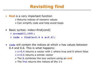
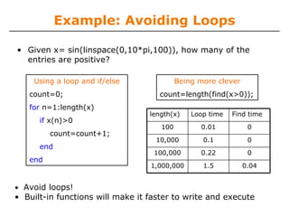
43. Efficient Code
• Avoid loops
This is referred to as vectorization
• Vectorized code is more efficient for MATLAB
• Use indexing and matrix operations to avoid loops
• For example, to sum up every two consecutive terms:
» a=rand(1,100);
» a=rand(1,100);
» b=[0 a(1:end-1)]+a;
» b=zeros(1,100);
Efficient and clean.
» for n=1:100
Can also do this using
»
if n==1
conv
»
b(n)=a(n);
»
else
»
b(n)=a(n-1)+a(n);
»
end
» end
Slow and complicated

44. End of Lecture 2
(1)
(2)
(3)
(4)
(5)
Functions
Flow Control
Line Plots
Image/Surface Plots
Vectorization
Vectorization makes
coding fun!

45. MIT OpenCourseWare
http://ocw.mit.edu
6.094 Introduction to MATLAB®
January (IAP) 2010
For information about citing these materials or our Terms of Use, visit: http://ocw.mit.edu/terms.