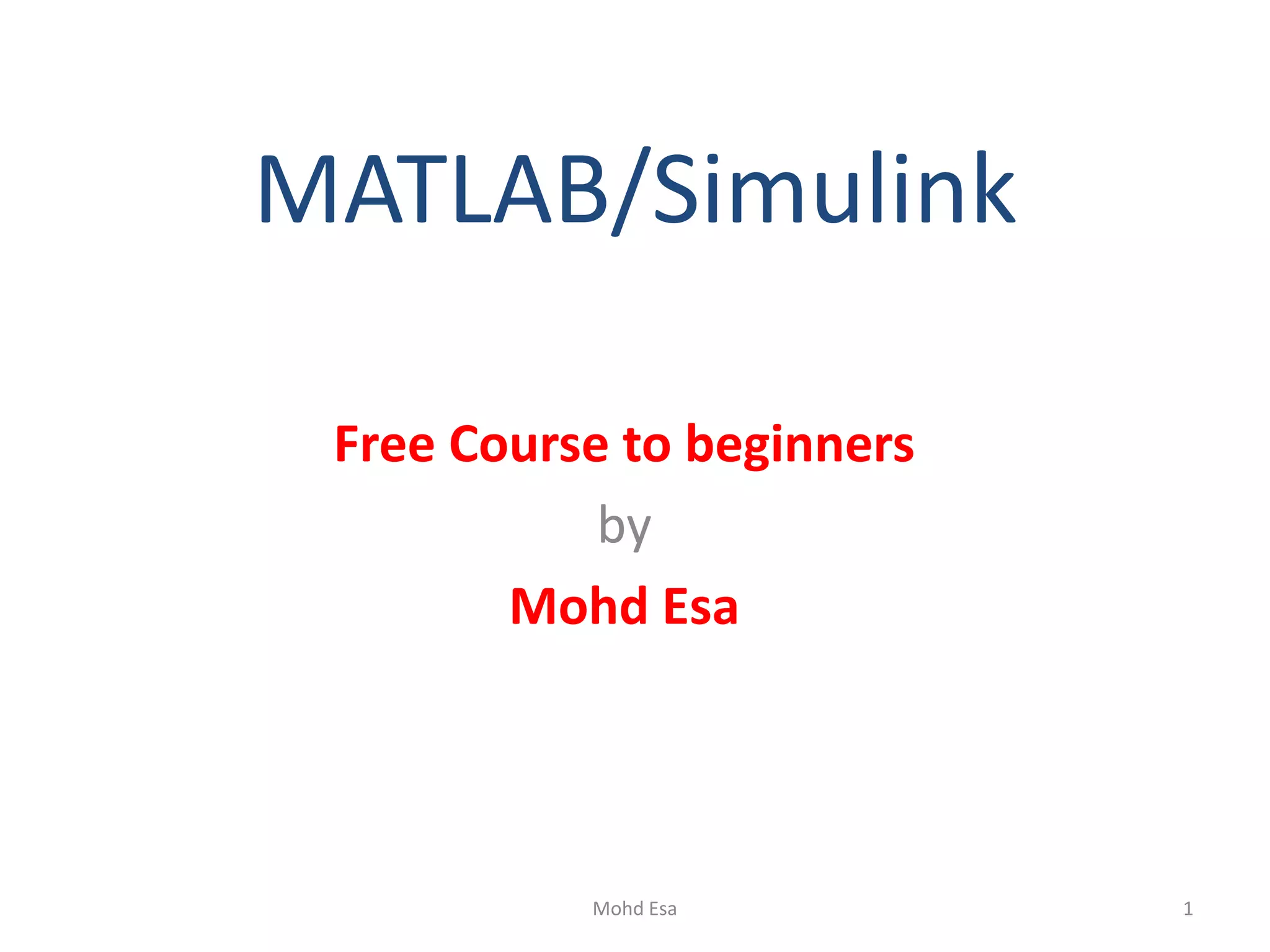

![Plotting Example-1
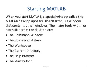
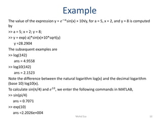
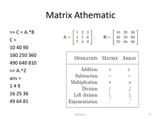
The MATLAB command to plot a graph is plot (x,y). The vectors x = (1, 2, 3, 4, 5, 6) and y = (3, −1,
2, 4, 5, 1) produce the picture shown
>> x = [1 2 3 4 5 6];
>> y = [3 -1 2 4 5 1];
>> plot(x,y)
13Mohd Esa](https://image.slidesharecdn.com/matlab-190907084011/85/Matlab-free-course-by-Mohd-Esa-13-320.jpg)
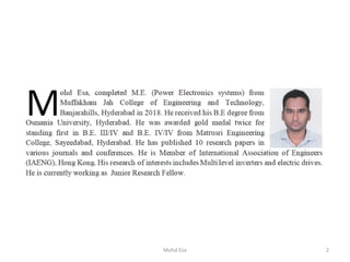
![Multiple data sets in one plot
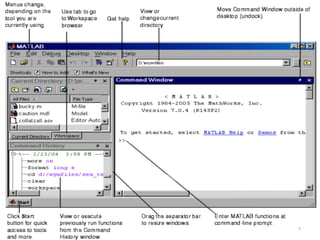
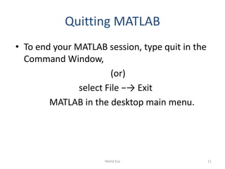
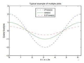
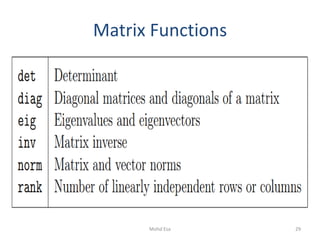
• Multiple (x, y) pairs arguments create multiple graphs with a single call to plot. For
example, these statements plot three related functions of x: y1 = 2 cos(x), y2 =
cos(x), and y3 = 0.5 ∗ cos(x), in the interval 0 ≤ x ≤ 2π.
>> x = 0:pi/100:2*pi;
>> y1 = 2*cos(x);
>> y2 = cos(x);
>> y3 = 0.5*cos(x);
>> plot(x,y1,’--’,x,y2,’-’,x,y3,’:’)
>> xlabel(’0 leq x leq 2pi’)
>> ylabel(’Cosine functions’)
>> legend(’2*cos(x)’,’cos(x)’,’0.5*cos(x)’)
>> title(’Typical example of multiple plots’)
>> axis([0 2*pi -3 3])
16Mohd Esa](https://image.slidesharecdn.com/matlab-190907084011/85/Matlab-free-course-by-Mohd-Esa-16-320.jpg)
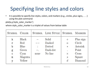
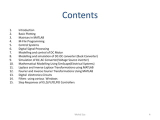
![Row & Column Vector
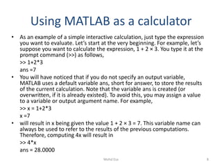
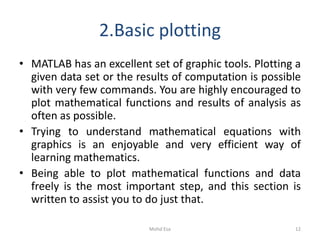
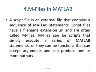
To enter a row vector, v, type
>> v = [1 4 7 10 13]
v = 1 4 7 10 13
Column vectors are created in a similar way, however, semicolon
(;) must separate the components of a column vector,
>> w = [1;4;7;10;13]
w =
1
4
7
10
13 20Mohd Esa](https://image.slidesharecdn.com/matlab-190907084011/85/Matlab-free-course-by-Mohd-Esa-20-320.jpg)
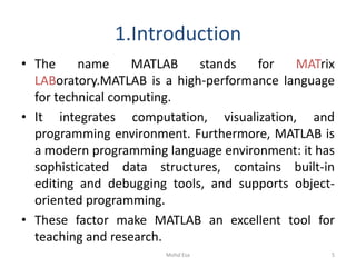
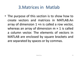
![Entering a matrix
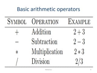
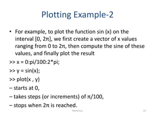
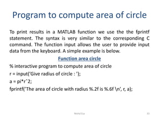
• A matrix is an array of numbers. To type a
matrix into MATLAB you must
• begin with a square bracket, [
• separate elements in a row with spaces or
commas (,)
• use a semicolon (;) to separate rows
• end the matrix with another square bracket, ]
22Mohd Esa](https://image.slidesharecdn.com/matlab-190907084011/85/Matlab-free-course-by-Mohd-Esa-22-320.jpg)
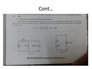
![Example
• Here is a typical example. To enter a matrix A,
such as,
>> A = [1 2 3; 4 5 6; 7 8 9]
• MATLAB then displays the 3 × 3 matrix as follows,
A =
1 2 3
4 5 6
7 8 9
23Mohd Esa](https://image.slidesharecdn.com/matlab-190907084011/85/Matlab-free-course-by-Mohd-Esa-23-320.jpg)
![Matrix inverse
• >> A = [1 2 3; 4 5 6; 7 8 0];
>> inv(A)
ans =
-1.7778 0.8889 -0.1111
1.5556 -0.7778 0.2222
-0.1111 0.2222 -0.1111
>> det(A)
ans =
27
28Mohd Esa](https://image.slidesharecdn.com/matlab-190907084011/85/Matlab-free-course-by-Mohd-Esa-28-320.jpg)
![Example-1 of M-File
• Use the MATLAB editor to create a file: File →
New → M-file.
A = [1 2 3; 3 3 4; 2 3 3];
b = [1; 1; 2];
x = Ab
Save the file, for example, example1.m.
• Run the file, in the command line, by typing:
>> example1
x =
-0.5000
1.5000
-0.5000
31Mohd Esa](https://image.slidesharecdn.com/matlab-190907084011/85/Matlab-free-course-by-Mohd-Esa-31-320.jpg)
![Example-2 of M-File(Same example previously
executed in command window)
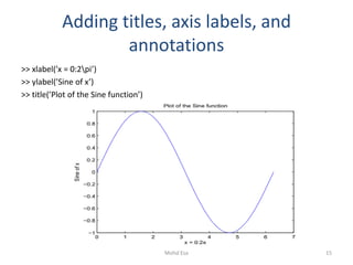
Plot the following cosine functions, y1 = 2 cos(x), y2 = cos(x), and y3 = 0.5 ∗
cos(x), in the interval 0 ≤ x ≤ 2π.
• Create a file, say example2.m, which contains the following commands
x = 0:pi/100:2*pi;
y1 = 2*cos(x);
y2 = cos(x);
y3 = 0.5*cos(x);
plot(x,y1,’--’,x,y2,’-’,x,y3,’:’)
xlabel(’0 leq x leq 2pi’)
ylabel(’Cosine functions’)
legend(’2*cos(x)’,’cos(x)’,’0.5*cos(x)’)
title(’Typical example of multiple plots’)
axis([0 2*pi -3 3])
Run the file by typing example2 in the Command Window.
32Mohd Esa](https://image.slidesharecdn.com/matlab-190907084011/85/Matlab-free-course-by-Mohd-Esa-32-320.jpg)
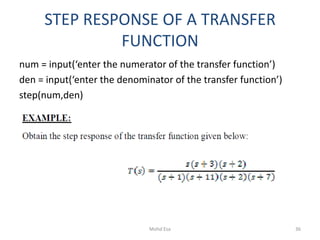
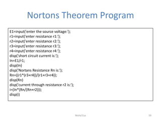
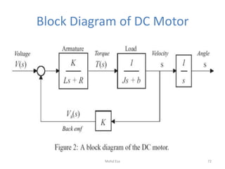
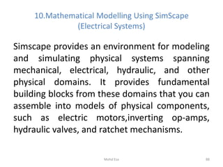
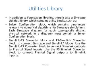
![5.Control Systems
TRANSFER FUNCTION FROM ZEROS AND POLES
MATLAB PROGRAM:
z=input(‘enter zeroes’)
p=input(‘enter poles’)
k=input(‘enter gain’)
[num,den]=zp2tf(z,p,k)
tf(num,den)
EXAMPLE:
Given poles are -3.2+j7.8,-3.2-j7.8,-4.1+j5.9,-4.1-j5.9,-8 and the zeroes are -
0.8+j0.43,-0.8-j0.43,-0.6 with a gain of 0.5
34Mohd Esa](https://image.slidesharecdn.com/matlab-190907084011/85/Matlab-free-course-by-Mohd-Esa-34-320.jpg)
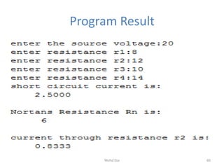
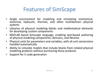
![ZEROS AND POLES FROM TRANSFER
FUNCTION
MATLAB PROGRAM:
num = input(‘enter the numerator of the transfer function’)
den = input(‘enter the denominator of the transfer function’)
[z,p,k] = tf2zp(num,den)
EXAMPLE:
35Mohd Esa](https://image.slidesharecdn.com/matlab-190907084011/85/Matlab-free-course-by-Mohd-Esa-35-320.jpg)
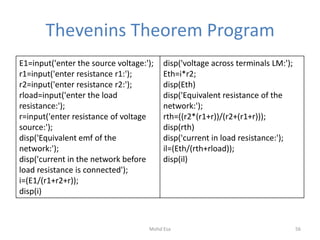
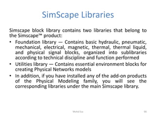
![BODE PLOT FROM A TRANSFER FUNCTION
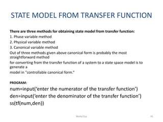
PROGRAM:
num=input('enter the numerator of the transfer function')
den=input('enter the denominator of the transfer function')
h=tf(num,den)
[gm pm wcp wcg]=margin(h)
bode(h)
39Mohd Esa](https://image.slidesharecdn.com/matlab-190907084011/85/Matlab-free-course-by-Mohd-Esa-39-320.jpg)
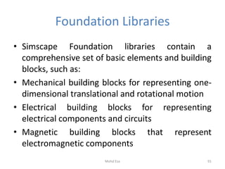
![STATE MODEL FROM ZEROS AND POLES
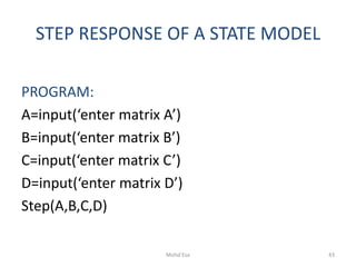
PROGRAM:
z=input('enter zeros')
p=input('enter poles')
k=input('enter gain')
[A,B,C,D]=zp2ss(z,p,k)
42Mohd Esa](https://image.slidesharecdn.com/matlab-190907084011/85/Matlab-free-course-by-Mohd-Esa-42-320.jpg)
![NYQUIST PLOT FROM TRANSFER
FUNCTION
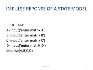
PROGRAM:
num=input(‘enter the numerator of the transfer function’)
den=input(‘enter the denominator of the transfer function’)
h=tf(num,den)
nyquist(h)
[gm pm wcp wcg]=margin(h)
if(wcp>wcg)
disp(‘system is stable’)
else
disp(‘system is unstable’)
end
46Mohd Esa](https://image.slidesharecdn.com/matlab-190907084011/85/Matlab-free-course-by-Mohd-Esa-46-320.jpg)
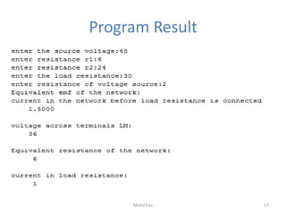
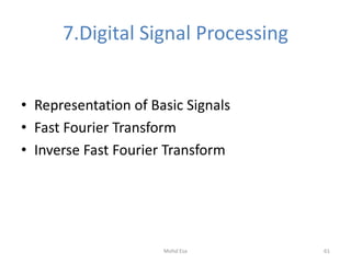
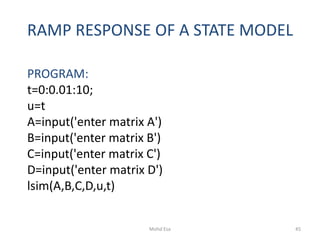
![Representation of basic signals
%Unit Impulse Signal%
n1=input('Enter the no of
samples');
x1=[-n1:1:n1];
y1=[zeros(1,n1),ones(1,1),zero
s(1,n1)];
subplot(2,3,1);
stem(x1,y1);
xlabel('Time Period');
ylabel('Amplitude');
title('Unit Impulse Signal');
%Unit Step Signal%
n2=input('Enter the no of
samples');
x2=[0:1:n2];
y2=ones(1,n2+1);
subplot(2,3,2);
stem(x2,y2);
xlabel('Time Period');
ylabel('Amplitude');
title('Unit Step Signal');
%Unit Ramp Signal%
n3=input('Enter the no of
samples');
x3=[0:1:n3];
subplot(2,3,3);
stem(x3,x3);
xlabel('Time Period');
ylabel('Amplitude');
title('Unit Ramp Signal');
%Exponential Signal%
n4=input('Enter the length of
the signal');
a=input('Enter the value of
a:');
x4=[0:1:n4];
y4=a*exp(x4);
subplot(2,3,4);
stem(x4,y4);
xlabel('Time Period');
ylabel('Amplitude');
title('Exponential Signal');
%Sinusoidal Signal%
x5=[-pi:0.1:pi];
y5=sin(2*pi*x5);
subplot(2,3,5);
plot(x5,y5);
xlabel('Time Period');
ylabel('Amplitude');
title('Sinusoidal Signal');
%Cosine Signal%
x6=[-pi:0.1:pi];
y6=cos(2*pi*x5);
subplot(2,3,6);
plot(x6,y6);
xlabel('Time Period');
ylabel('Amplitude');
title('Cosine Signal')
62Mohd Esa](https://image.slidesharecdn.com/matlab-190907084011/85/Matlab-free-course-by-Mohd-Esa-62-320.jpg)

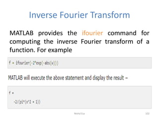
![12.Fourier and Inverse Fourier
transformations Using MATLAB
Program For Fourier Transformation
syms x
f = exp(-2*x^2); %our function
ezplot(f,[-2,2]) % plot of our function
FT = fourier(f) % Fourier transform
The following result is displayed −
FT =
(2^(1/2)*pi^(1/2)*exp(-w^2/8))/2
Plotting the Fourier transform as −
ezplot(FT)
101Mohd Esa](https://image.slidesharecdn.com/matlab-190907084011/85/Matlab-free-course-by-Mohd-Esa-101-320.jpg)
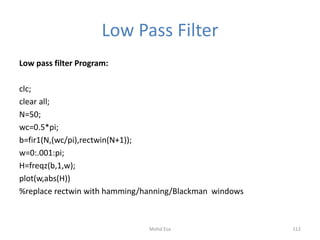
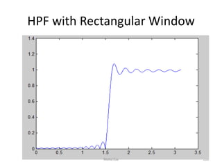
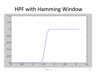
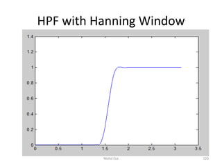
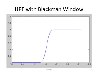
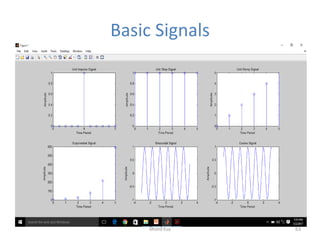
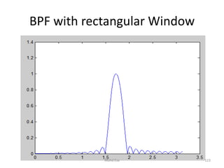
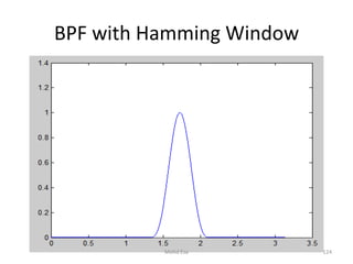
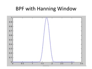
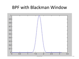
![Band Pass Filter
clc;
clear all;
N=50;
wc1=0.5*pi;
wc2=0.6*pi;
b=fir1(N,[wc1/pi,wc2/pi],'bandpass',rectwin(N+1));
w=0:.001:pi;
H=freqz(b,1,w);
plot(w,abs(H))
%replace rectwin with hamming/hanning/Blackman windows
122Mohd Esa](https://image.slidesharecdn.com/matlab-190907084011/85/Matlab-free-course-by-Mohd-Esa-122-320.jpg)
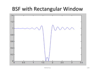
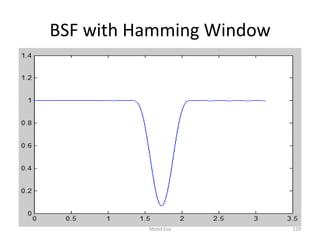
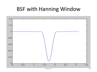
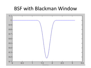
![Band Stop Filter
clc;
clear all;
N=50;
wc1=0.5*pi;
wc2=0.6*pi;
b=fir1(N,[wc1/pi,wc2/pi],'stop',rectwin(N+1));
w=0:.001:pi;
H=freqz(b,1,w);
plot(w,abs(H))
%replace rectwin with hamming/hanning/Blackman windows
127Mohd Esa](https://image.slidesharecdn.com/matlab-190907084011/85/Matlab-free-course-by-Mohd-Esa-127-320.jpg)
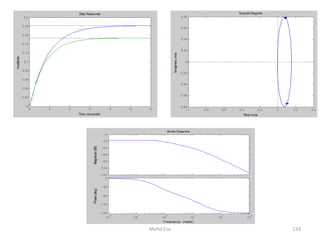
![Step Responses of P,I,D,PI,PD,PID
Controllers
P Controller (kp=1)
clc
clear all
close all
kp=input('enter the value of kp');
num=[1+kp];
den=[1,20,10+kp];
h=tf(num,den);
step(h)
figure
g=feedback(h,1);
step(g)
figure
step(h,g)
figure
nyquist(g)
figure
bode(g)
132Mohd Esa](https://image.slidesharecdn.com/matlab-190907084011/85/Matlab-free-course-by-Mohd-Esa-132-320.jpg)
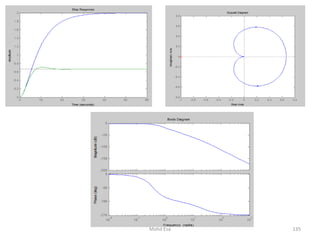
![I Controller(ki=1)
clc
clear all
close all
ki=input('enter the value of ki');
num=[1+ki];
den=[1,20,10,ki];
h=tf(num,den);
step(h)
figure
g=feedback(h,1);
step(g)
figure
step(h,g)
figure
nyquist(g)
figure
bode(g) 134Mohd Esa](https://image.slidesharecdn.com/matlab-190907084011/85/Matlab-free-course-by-Mohd-Esa-134-320.jpg)
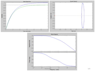
![D Controller(kd=1)
clc
clear all
close all
kd=input('enter the value of kd');
num=1;
den=[1,(20+kd),10];
h=tf(num,den);
step(h)
figure
g=feedback(h,1);
step(g)
figure
step(h,g)
figure
nyquist(g)
figure
bode(g) 136Mohd Esa](https://image.slidesharecdn.com/matlab-190907084011/85/Matlab-free-course-by-Mohd-Esa-136-320.jpg)
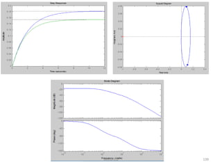
![PD Controller (kp=1;kd=2)
clc
clear all
close all
kd=input('enter the value of kd');
kp=input('enter the value of kp');
num=1+kp;
den=[1,20+kd,10+kp];
h=tf(num,den);
step(h)
figure
g=feedback(h,1);
step(g)
figure
step(h,g)
figure
nyquist(g)
figure
bode(g)
138Mohd Esa](https://image.slidesharecdn.com/matlab-190907084011/85/Matlab-free-course-by-Mohd-Esa-138-320.jpg)
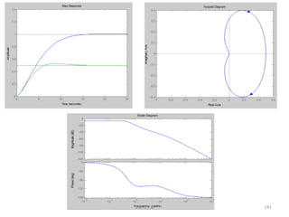
![PI Controller(kp=1,ki=2)
clc
clear all
close all
kp=input('enter the value of kp');
ki=input('enter the value of ki');
num=[kp,ki];
den=[1,20,10+kp,ki];
h=tf(num,den);
step(h)
figure
g=feedback(h,1);
step(g)
figure
step(h,g)
figure
nyquist(g)
figure
bode(g)
140Mohd Esa](https://image.slidesharecdn.com/matlab-190907084011/85/Matlab-free-course-by-Mohd-Esa-140-320.jpg)
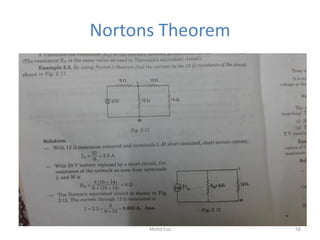
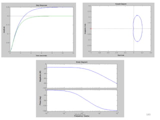
![PID Controller (kp=1;ki=2;kd=3)
clc
clear all
close all
kp=input('enter the value of kp');
ki=input('enter the value of ki');
kd=input('enter the value of kd');
num=[1+ki];
den=[1+kd,20+kp,10+ki];
h=tf(num,den);
step(h)
figure
g=feedback(h,1);
step(g)
figure
step(h,g)
figure
nyquist(g)
figure
bode(g)
142Mohd Esa](https://image.slidesharecdn.com/matlab-190907084011/85/Matlab-free-course-by-Mohd-Esa-142-320.jpg)


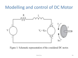
The document is a comprehensive guide to MATLAB and Simulink, aimed at beginners, covering various fundamental topics including basic plotting, matrix operations, m-file programming, control systems, and digital signal processing. It provides step-by-step instructions and examples for using MATLAB's features, such as creating vectors and matrices, plotting functions, and executing scripts. Additionally, it includes sections on control system analysis and circuit theorems, showcasing MATLAB's application in engineering fields.