Download to read offline


![MATLAB Matrices
A matrix with only one row is called a row vector. A row vector can be
created in MATLAB as follows (note the commas):
» rowvec = [12 , 14 , 63]
rowvec =
12 14 63
A matrix with only one column is called a column vector. A column
vector can be created in MATLAB as follows (note the semicolons):
» colvec = [13 ; 45; -2]
colvec =
13
45
-2](https://image.slidesharecdn.com/presentation-240129160049-cd11c5df/85/INTRODUCTION-TO-MATLAB-presentation-pptx-6-320.jpg)
![MATLAB Matrices
A matrix can be created in MATLAB as follows (note the commas
AND semicolons):
» matrix = [1 , 2 , 3 ; 4 , 5 ,6 ; 7 , 8 , 9]
matrix =
1 2 3
4 5 6
7 8 9](https://image.slidesharecdn.com/presentation-240129160049-cd11c5df/85/INTRODUCTION-TO-MATLAB-presentation-pptx-7-320.jpg)
![Index
MATLAB index starts with 1, NOT 0!
Vector Index:
◦ a = [22 17 7 4 42]
a(1) = 22
a(3) = 7
Matrix Index:
◦ a = [7 12 42; 5 1 23; 4 9 10];
a(1, 3) = 42
a(3, 2) = 9](https://image.slidesharecdn.com/presentation-240129160049-cd11c5df/85/INTRODUCTION-TO-MATLAB-presentation-pptx-8-320.jpg)
![Some matrix functions in MATLAB
X = ones(r,c) Creates matrix full with ones
X = zeros(r,c) Creates matrix full with zeros
A = diag(x) Creates squared matrix with vector x in diagonal
[r,c] = size(A) Return dimensions of matrix A
X = A’ Transposed matrix
X = inv(A) Inverse matrix squared matrix
X = pinv(A) Pseudo inverse
d = det(A) Determinant
[X,D] = eig(A) Eigenvalues and eigenvectors
[U,D,V] = svd(A) singular value decomposition](https://image.slidesharecdn.com/presentation-240129160049-cd11c5df/85/INTRODUCTION-TO-MATLAB-presentation-pptx-9-320.jpg)
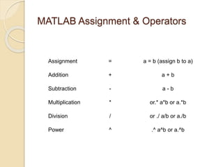
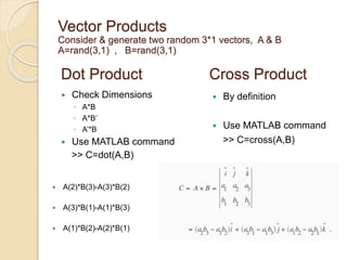
![Dot Operator
For scalar operations, nothing new is needed. Example:
a = 5; b = 3; ==> c = a*b %c = 15
For element operations, a dot must be used before the operator.
Note: Dot operator not the same as dot product!
Example:
◦ a = [1 2 3 4];
◦ b = [5 6 7 8];
◦ c = a*b
◦ Result: ??? Error using ==> mtimes
inner matrix dimensions must agree
Now, try:
◦ c = a.*b %notice the dot!
◦ Result: c=[5 12 21 32]
Notice what it is doing: a(1)*b(1), a(2)*b(2), etc.](https://image.slidesharecdn.com/presentation-240129160049-cd11c5df/85/INTRODUCTION-TO-MATLAB-presentation-pptx-10-320.jpg)

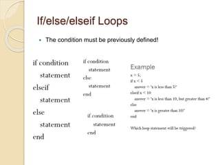


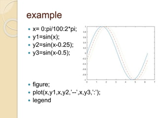
![Axis-specific
Helps focus on what is important on the graph.
Change only the x or y axis limits:
◦ xlim([xminxmax]) or ylim([yminymax])
◦ min and max can be positive or negative.
example](https://image.slidesharecdn.com/presentation-240129160049-cd11c5df/85/INTRODUCTION-TO-MATLAB-presentation-pptx-23-320.jpg)

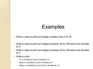
![plotyy
2D line plots with y-axis on both left and right side
◦ [AX,H1,H2]=plotyy(x1,y1,x2,y2)](https://image.slidesharecdn.com/presentation-240129160049-cd11c5df/85/INTRODUCTION-TO-MATLAB-presentation-pptx-25-320.jpg)

![Polynomials
We can use an array to represent a polynomial. To do so we
use list the coefficients in decreasing order of the powers. For
example x3+4x+15 will look like [1 0 4 15]
To find roots of this polynomial we use roots command. roots
([1 0 4 15])
To create a polynomial from its roots poly command is used.
poly([1 2 3]) where r1=1, r2=2, r3=3
To evaluate the new polynomial at x =5 we can use polyval
command. polyval([ 1 -6 11 -6], 5)](https://image.slidesharecdn.com/presentation-240129160049-cd11c5df/85/INTRODUCTION-TO-MATLAB-presentation-pptx-28-320.jpg)
![Systems of Equations
Consider the following system of equations
◦ x+5y+15z=7
◦ x-3y+13z=3
◦ 3x-4y-15z=11
One way to solve this system of equations is to use matrices.
First, define matrix A:
◦ A=[1 5 15; 1 -3 13; 3 -4 15];
Second, matrix b:
◦ b=[7;3;11];
Third, we solve the equation Ax=b for x, taking the inverse of A
and multiply it by b:
◦ x=inv(A)*b
Note that we cannot solve equation Ax=b by dividing b by A
because vectors A and b have different dimensions!](https://image.slidesharecdn.com/presentation-240129160049-cd11c5df/85/INTRODUCTION-TO-MATLAB-presentation-pptx-29-320.jpg)
![Systems of Equations
Consider the following system of equations
◦ x+5y+15z=7
◦ x-3y+13z=3
◦ 3x-4y-15z=11
One way to solve this system of equations is to use matrices.
First, define matrix A:
◦ A=[1 5 15; 1 -3 13; 3 -4 15];
Second, matrix b:
◦ b=[7;3;11];
Third, we solve the equation Ax=b for x, taking the inverse of A
and multiply it by b:
◦ x=inv(A)*b
Note that we cannot solve equation Ax=b by dividing b by A
because vectors A and b have different dimensions!](https://image.slidesharecdn.com/presentation-240129160049-cd11c5df/85/INTRODUCTION-TO-MATLAB-presentation-pptx-31-320.jpg)
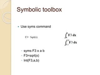


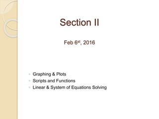
![Solving ODE with dsolve,
systems
Systems of equations
◦ EQs:
[x,y,z]=dsolve(’Dx=x+2*y-z’,’Dy=x+z’,’Dz=4*x-4*y+5*z’)
inits=’x(0)=1,y(0)=2,z(0)=3’;
[x,y,z]=dsolve(’Dx=x+2*y-z’,’Dy=x+z’,’Dz=4*x-4*y+5*z’,inits)
Notice that since no independent variable was specified,
MATLAB used its default, t.
◦ Plotting
t=linspace(0,.5,25);
xx=eval(vectorize(x));
yy=eval(vectorize(y));
zz=eval(vectorize(z));
plot(t, xx, t, yy, t, zz)](https://image.slidesharecdn.com/presentation-240129160049-cd11c5df/85/INTRODUCTION-TO-MATLAB-presentation-pptx-36-320.jpg)


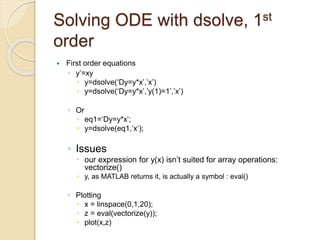
![Solving first-order ODEs
Define the function M-file
function y_dot=EOM(y,t)
global alpha gamma
y_dot=alpha * y - gamma * y^2;
end
Make a script M-file
global alpha gamma
alpha=0.15;
gamma=3.5;
y0=1;
[y t]=ode45(@EOM,[0 10],y0);
plot(t,y);](https://image.slidesharecdn.com/presentation-240129160049-cd11c5df/85/INTRODUCTION-TO-MATLAB-presentation-pptx-41-320.jpg)


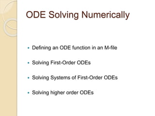
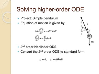
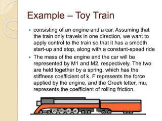
![Example
Use “ode45” to solve the following differential
equation and plot y(x) in the interval of [0,6π]. Put
your name in the plot title.](https://image.slidesharecdn.com/presentation-240129160049-cd11c5df/85/INTRODUCTION-TO-MATLAB-presentation-pptx-44-320.jpg)
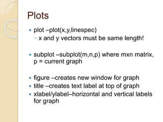
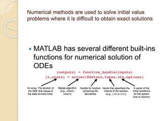
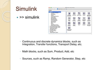
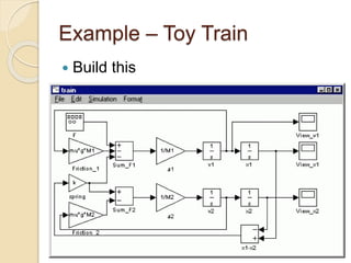
![Simple Pendulum
Initial conditions and constants
Coding
◦ Make a function M-file for equation of motion
function z_dot=EOM_pendulum(t,z)
global G L
theta=z(1);
theta_dot=z(2);
theta_dot2=-(G/L)*sin(theta);
z_dot=[theta_dot;theta_dot2];
end
◦ Make a script M-file to run the code
global G L
G=9.8;
L=2;
tspan=[0 2*pi];
inits=[pi/3 0];
[t, y]=ode45(@EOM_pendulum,tspan,inits);](https://image.slidesharecdn.com/presentation-240129160049-cd11c5df/85/INTRODUCTION-TO-MATLAB-presentation-pptx-46-320.jpg)
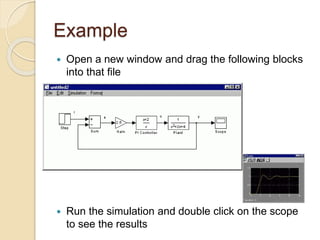
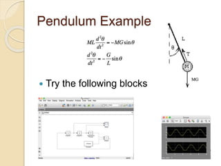
![Lorenz Equations
Initials and constants, T=[0 20]
Plot x vs. z , check if you
get same results as](https://image.slidesharecdn.com/presentation-240129160049-cd11c5df/85/INTRODUCTION-TO-MATLAB-presentation-pptx-47-320.jpg)


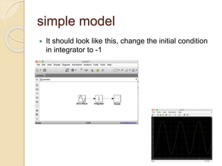


Here are the steps to solve this problem numerically in MATLAB: 1. Define the 2nd order ODE for the pendulum as two first order equations: y1' = y2 y2' = -sin(y1) 2. Create an M-file function pendulum.m that returns the right hand side: function dy = pendulum(t,y) dy = [y(2); -sin(y(1))]; end 3. Use an ODE solver like ode45 to integrate from t=0 to t=6pi with initial conditions y1(0)=pi, y2(0)=0: [t,y] = ode45