Downloaded 22 times
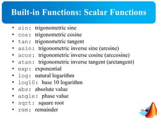
![Vectors
• Vector in space
𝑍 = 2 𝑎 𝑥 + 3 𝑎 𝑦 + 7 𝑎 𝑧
• Can be written as
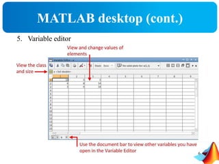
• Use ‘space’ (‘ ’) or ‘comma’ (‘,’) to separate row elements.
• Use ‘semicolon’ (‘;’) to separate rows.
• Define a row vector ‘r’ and column vector ‘c’.
• If we no longer need a particular variable/vector/
/matrix/object we can “erase” it from memory using the
command ‘clear variable_name’.
• Erase vector ‘r’.
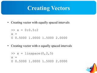
2 3 7
or
2
3
7
Row vector Column vector
>> r = [1 2 3 4 5]; or r = [1,2,3,4,5];
>> c = [6;7;8;9;10];
10](https://image.slidesharecdn.com/matlabtraining1-150608122116-lva1-app6892/85/Lines-and-planes-in-space-10-320.jpg)
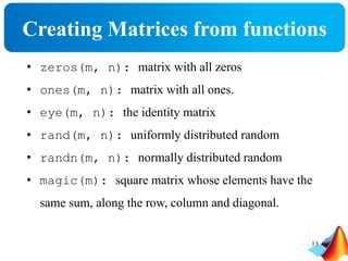
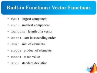
![Matrices
• Almost all entities in MATLAB are matrices.
• Order of Matrix − m × n
m = number of rows
n = number of rows
• Vectors are special case of Matrices
− m = 1 row vector
− n = 1 column vector
• Define
• A vector is always a matrix but a matrix is not necessarily a
vector
• Use ‘size (variable/vector/matrix name)’ to find its size.
>> A = [1 2; 3 4]
>> B = [16 3 5; 7 5 10]
11](https://image.slidesharecdn.com/matlabtraining1-150608122116-lva1-app6892/85/Lines-and-planes-in-space-11-320.jpg)
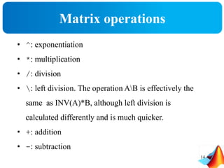
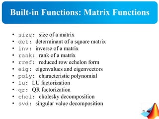
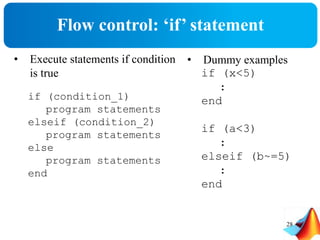
![Example
Perform the following task.
• Define matrices ‘A’ and ‘B’
>> A=[1 2;3 4];
>> B=[5 6;7 8];
Find product of ‘A’ and ‘B’ using Matrix and Array
operator.
Which one is correct??
Hint: Solve on paper before using MATLAB
16](https://image.slidesharecdn.com/matlabtraining1-150608122116-lva1-app6892/85/Lines-and-planes-in-space-16-320.jpg)
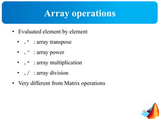
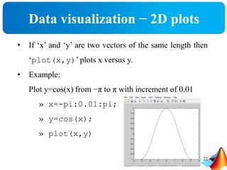
![Matrix Indexing
Given the matrix:
Then:
A(1,2) = 0.6068
A(3) = 0.6068
A(:,1) = [0.9501
0.2311 ]
A(1,2:3)=[0.6068 0.4231]
𝐴 =
0.9501 0.6068 0.4231
0.2311 0.4860 0.2774
17](https://image.slidesharecdn.com/matlabtraining1-150608122116-lva1-app6892/85/Lines-and-planes-in-space-17-320.jpg)
![Adding Elements to a Vector or a Matrix
>> C=[1 2; 3 4]
C=
1 2
3 4
>> C(3,:)=[5 6];
C=
1 2
3 4
5 6
>> D=linspace(4,12,3);
>> E=[C D’]
E=
1 2 4
3 4 8
5 6 12
>> A=1:3
A=
1 2 3
>> A(4:6)=5:2:9
A=
1 2 3 5 7 9
>> B=1:2
B=
1 2
>> B(5)=7;
B=
1 2 0 0 7
18](https://image.slidesharecdn.com/matlabtraining1-150608122116-lva1-app6892/85/Lines-and-planes-in-space-18-320.jpg)
![2D plots − Annotation
• Use title, xlabel, ylabel and legend for
annotation
Example
>> title('Demo plot');
>> xlabel('X Axis');
>> ylabel('Y Axis');
>> legend([pl, p2], 'x^2', 'x^3');
24](https://image.slidesharecdn.com/matlabtraining1-150608122116-lva1-app6892/85/Lines-and-planes-in-space-24-320.jpg)
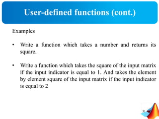
![User-defined functions
30
• Functions are m-files which can be executed by
specifying some inputs and supply some desired
outputs.
function output = functionname(inputs)
function [out1,out2,…] = functionname(in1,in2…)
• Write this command at the beginning of the m-file and save the
m-file with a file name same as the function name.](https://image.slidesharecdn.com/matlabtraining1-150608122116-lva1-app6892/85/Lines-and-planes-in-space-30-320.jpg)

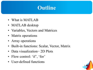
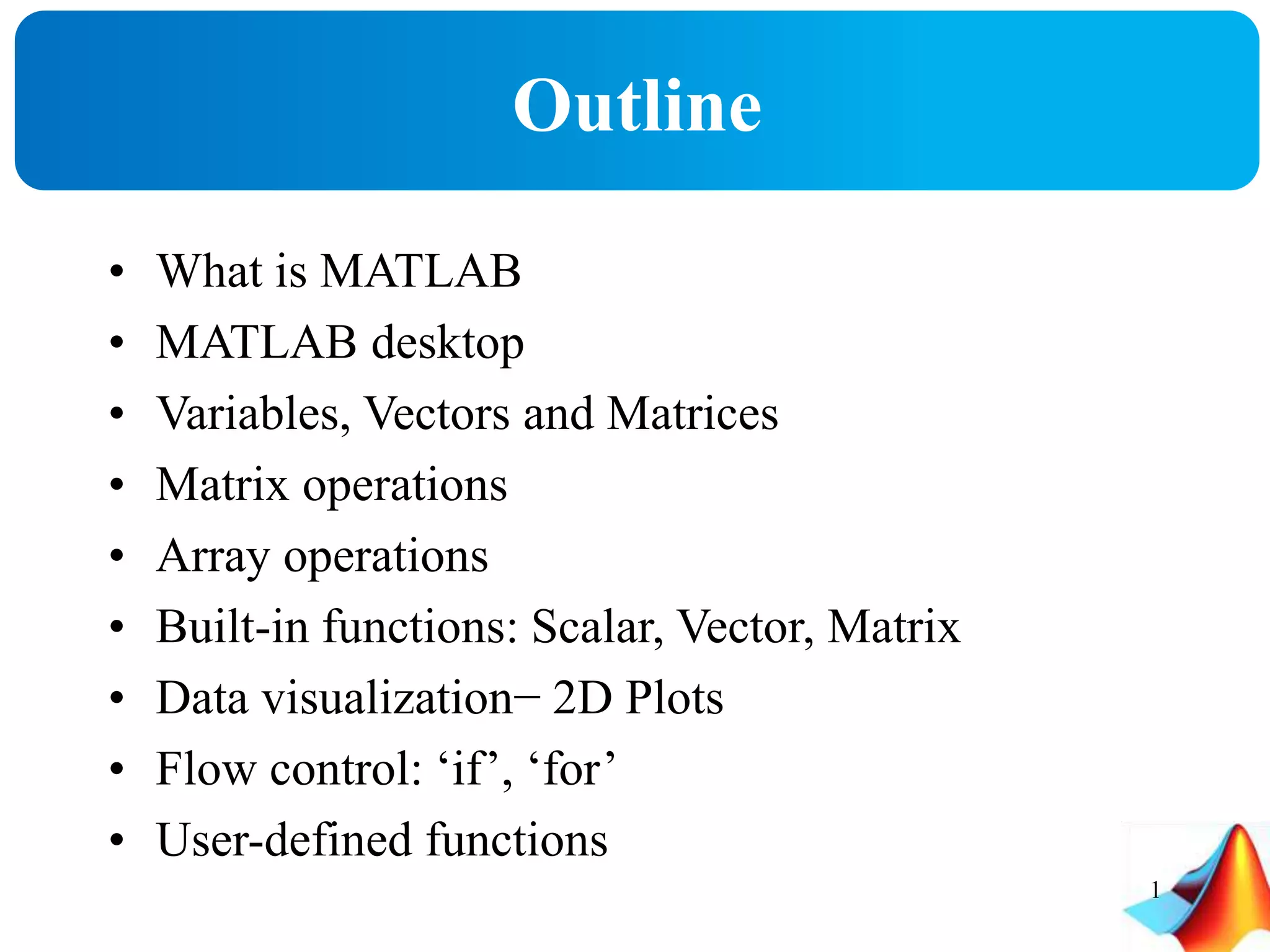
This document provides an overview of MATLAB, including the MATLAB desktop, variables, vectors, matrices, matrix operations, array operations, built-in functions, data visualization, flow control using if and for statements, and user-defined functions. It introduces key MATLAB concepts like the command window, workspace, and editor. It also demonstrates how to create and manipulate variables, vectors, matrices, and plots in MATLAB.