1) The document describes designing a microstrip transmission line in HFSS software to meet specified objectives. Key steps included drawing the substrate and ground plane boxes, assigning the microstrip width, adding wave ports, enclosing in a radiation box, and simulating the design.
2) Field plots and S-parameter results were analyzed to verify the design met expectations. The port impedance and total loss were also checked.
3) Objectives of introducing HFSS software, designing a basic microstrip structure, assigning wave ports, building a radiation box, and analyzing simulation results were achieved.
This document discusses Ansoft HFSS simulation software. It provides an overview of HFSS's main features like automatic adaptive meshing and advanced finite element method technology. It also describes getting started with HFSS, provides an example of simulating a microstrip patch antenna, and lists advantages like high productivity for research and development. The document concludes that HFSS is well-suited for simulating planar antennas and designing complex RF components.
Microstrip transmission lines are used extensively in microwave integrated circuits. They consist of a conducting strip separated from a ground plane by a dielectric substrate and support a quasi-TEM wave. Microstrip lines can be easily fabricated using printed circuit board technology. Their characteristic impedance depends on the strip width, thickness, distance to the ground plane, and dielectric constant of the substrate material. Microstrip lines are used for interconnecting high-speed circuits due to their uniform signal paths and ability to be fabricated automatically, though they have higher radiation losses than other transmission line types.
Design & Study of Microstrip Patch Antenna.The project here provides a detailed study of how to design a probe-fed Square Micro-strip Patch Antenna using HFSS, v11.0 software and study the effect of antenna dimensions Length (L), and substrate parameters relative Dielectric constant (εr), substrate thickness (t) on the Radiation parameters of Bandwidth and Beam-width.
Design and Simulation Microstrip patch Antenna using CST Microwave StudioAymen Al-obaidi
The document describes the design and simulation of a microstrip patch antenna in CST Microwave Studio. It begins with an introduction to microstrip patch antennas and their applications. Then, it outlines the theoretical design of a rectangular patch antenna for 2.4 GHz WiFi using transmission line equations. Finally, it details the simulation process in CST Microwave Studio, including adding the patch, feedline, substrate and ground plane, assigning materials and frequencies, setting up the port and monitors, and solving to obtain results like the bandwidth and radiation pattern.
1) The document presents information about a magic tee, which is a waveguide component used in microwave engineering systems.
2) A magic tee has four ports and is able to split or combine signals passing through in specific ways depending on which port is used.
3) The document discusses the working, operation, and S-matrix of a magic tee. It also provides examples of how magic tees can be used for applications like impedance measurement, duplexing, and mixing.
Rectangular Microstrip Antenna Parameter Study with HFSSOmkar Rane
This document describes the design and parametric study of a rectangular microstrip patch antenna (MSA) using HFSS software. Key points:
- MSA design involves calculating the patch width and length based on the operating frequency, substrate properties. An MSA with dimensions of 16.597mm x 12.438mm was designed to operate at 5.5GHz.
- A parametric study was conducted by varying the patch dimensions and substrate properties to analyze their effect on performance. This included increasing/decreasing patch size, changing substrate height and material.
- MSAs have applications in mobile/satellite communications, GPS, RFID, WiMax, radar, and telemedicine due to their low profile,
This slide describes design and simulation about the micro strip patch antenna using HFSS software.study the return characteristics,gain(db)and radiation pattern
As the given frequency & substrate thickness, we calculate substrate length,width & patch length.you can refer theory in "ANTENNA THEORY" by C.A.Balanis
Amit Kirti Saran and Ramit Kirti Saran presented a design for a microstrip patch antenna at 2.45GHz. They described the basic structure of a microstrip patch antenna and the design equations used to calculate the patch dimensions. They then outlined the steps taken to design the patch antenna using HFSS software, including assigning the calculated values and adding an inset feed. Simulation results showed the radiation patterns and return loss of the designed antenna. Applications of microstrip patch antennas include mobile/satellite communication, GPS, Bluetooth, and medical and radar uses.
HFSS MICROSTRIP PATCH ANTENNA- ANALYSIS AND DESIGNShivashu Awasthi
This document describes the design and simulation of a microstrip patch antenna in Ansoft HFSS. It discusses the basic components of a microstrip patch antenna including the radiating patch, dielectric substrate and ground plane. It then covers the simulation process in HFSS including defining the geometry, materials, boundary conditions, excitation source and frequency sweep setup. The document concludes that a rectangular patch antenna was successfully designed and simulated in HFSS to operate at 2.55 GHz.
Microwave semiconductor devices include transistors, diodes, and detectors used in microwave systems. Bipolar junction transistors (BJTs) and field effect transistors (FETs) like MESFETs are commonly used in microwave applications. Schottky diodes have lower capacitance than PN junction diodes, making them suitable for microwave frequencies. Tunnel diodes exhibit negative resistance, allowing their use in microwave oscillators. PIN diodes have an intrinsic region that reduces junction capacitance. These devices are used in microwave systems for applications like amplification, mixing, and detection.
This document discusses carrier synchronization techniques in digital communication systems. It begins with an introduction to the need for carrier recovery and symbol synchronization at the receiver. It then covers maximum likelihood estimation of signal parameters including carrier phase. Next, it describes carrier phase estimation using a phase-locked loop and decision-directed loops. It explains how the phase-locked loop works to continuously track and update the carrier phase estimate. Finally, it provides an example of decision-directed carrier phase estimation for a double-sideband suppressed carrier pulse amplitude modulation signal.
Impedance matching is a procedure for obtaining the maximum power transfer to a load. What is a goal for microwave design? If we can give maximum power to a load, we succeed in design. Impedance matching allows us to make that happen.
1. Design a single stub shunt tuning network to match a 50Ω transmission line to a load impedance of 60-j80Ω at 2GHz using an FR4 substrate. Simulate the return loss in Microwave Office.
2. Design a double stub shunt tuner matching a 60-j80Ω load to a 50Ω line at 2GHz using open-circuited stubs spaced λ/8 apart on an FR4 substrate. Simulate the return loss.
3. Design an L-section matching network to match a 200-j100Ω series RC load to 100Ω at 500MHz on an FR4 substrate. Simulate the return loss.
This document provides an overview of analog communication systems and modulation techniques. It discusses the basic components of communication systems including the transmitter, transmission channel, receiver, and transducers. It then describes analog modulation methods like amplitude modulation (AM) and frequency modulation (FM) and how they vary the amplitude or frequency of a carrier wave to transmit a baseband signal. Digital modulation techniques like amplitude-shift keying (ASK) and frequency-shift keying (FSK) are also introduced. Modems are defined as devices that enable data transfer over analog networks by modulating and demodulating signals.
MMICs (Monolithic Microwave Integrated Circuits) are integrated circuits that operate at microwave frequencies between 300 MHz and 300 GHz. They are built on a single crystal and perform functions like microwave mixing, power amplification, and high frequency switching. MMICs are small, mass producible, and easier to use than hybrid circuits since they do not require external matching networks. They have advantages like low cost, small size, high reliability, and improved reproducibility. Some applications of MMICs include communications, homeland security scanners, imaging and sensors, and new areas like automotive radar and aircraft systems.
This document summarizes the two-ray propagation model used in wireless communications. It assumes both a line-of-sight signal and a reflected signal propagate between the transmitter and receiver. The key parameters estimated are the electric field of each ray, the path difference between them, the phase difference, and time delay. Using geometry, the path difference is derived as approximately equal to 2 times the transmitter and receiver heights divided by the separation distance. The phase difference and time delay are then defined in terms of this path difference. Finally, the total electric field is written as the sum of the individual LOS and reflected signal fields.
The document discusses the TRAPATT diode, which is a type of p-n junction diode that generates microwaves. It operates by forming a trapped plasma within the junction region when a high electric field propagates through. Key points:
- It was first reported in 1967 and can generate power over 1 kW at frequencies up to 50 GHz with efficiencies up to 75%
- It operates by inducing avalanche breakdown to generate a dense plasma of electrons and holes within the depletion region, which becomes trapped and oscillates the voltage and current
- Applications include low power Doppler radars, radio altimeters, and radar transmitters due to its pulsed operation capabilities between 3-50 GHz
MicroStrip Antenna
Introduction .
Micro-Strip Antennas Types .
Micro-Strip Antennas Shapes .
Types of Substrates (Dielectric Media) .
Comparison of various types of flat profile printed antennas .
Advantages & DisAdvantages of MSAs .
Applications of MSAs .
Radiation patterns of MSAs .
How to Optimizing the Substrate Properties for Increased Bandwidth ?
Comparing the different feed techniques .
In digital modulation, minimum-shift keying(MSK) is a type of continuous-phase frequency-shift keying that was developed in the late 1950s and 1960s.
Similar to OQPSK(Offset quadrature phase-shift keying),
This document discusses various applications of antennas in medical fields. It describes how antennas are used for wireless body area networks to transmit biomedical data from sensors on or inside the body to devices for diagnosis. Ingestible antennas inside capsules and wearable antennas on the body are discussed. Antennas are also used for medical imaging like MRI and microwave imaging. The document outlines how antennas can be designed and implemented for these diagnostic and therapeutic applications like thermal ablation treatment.
This presentation discusses MOSFET scaling and its challenges. It begins by covering Moore's Law, which states that the number of transistors on a chip doubles every 18 months. As sizes shrink due to scaling, short channel effects like drain-induced barrier lowering and hot carrier effects emerge. The presentation covers two types of scaling: constant field scaling, which keeps electric fields constant but increases power density; and constant voltage scaling, which is preferred as it avoids increased power density but reduces threshold voltage. Narrow width effects also occur when channel widths shrink and depletion regions overlap. Overall, the presentation provides an overview of MOSFET scaling techniques and the short channel effects that emerge as sizes shrink.
The document discusses various types of aperture antennas including slot antennas, horn antennas, and corrugated horns. It explains key concepts such as Babinet's principle, which relates the fields of an antenna to its complement, and how this allows the fields of a slot antenna to be understood based on a dipole antenna. The document also discusses how horns are commonly used as feeds for large satellite and radio astronomy dishes due to their simplicity, versatility, and ability to produce a uniform phase front. Corrugated horns are highlighted as a type of horn that can improve the aperture efficiency of large reflectors.
Synchronization is critical for communication systems with coherent receivers. There are three main types of synchronization: carrier synchronization, symbol/bit synchronization, and frame synchronization. Carrier synchronization compensates for frequency and phase differences between the received and local carrier waves. Symbol/bit synchronization samples the received signal at the symbol rate. Frame synchronization detects the start/stop times of data frames. Phase-locked loops (PLLs) are commonly used for carrier and symbol synchronization. There are various techniques for carrier synchronization extraction, including pilot tone insertion and direct extraction methods like square law detection and Costas loops. Barker codes and pseudo-random codes can provide frame alignment signals.
This document discusses various wireless propagation channels including free space propagation, reflection, scattering, and diffraction. It covers reflection propagation mechanisms such as reflection from dielectrics and conductors. Reflection coefficients and Snell's law are explained. Models for reflection, including the two-ray ground reflection model, are provided. Diffraction models like knife-edge diffraction and multiple knife-edge diffraction using methods like Bollington's method are summarized. Scattering models including Kirchoff's theory and perturbation theory are covered. Common fading models for mobile radio like Rayleigh, Rician, and Doppler shift models are described. Finally, different types of wireless channels including time-selective, frequency-selective, general, and WSSUS channels are classified
This document discusses MOSFET fabrication and thin-film formation processes. It describes the basic MOSFET fabrication steps including oxidation, diffusion, etching, and metallization. It also discusses NMOS and CMOS development processes. For thin-film formation, it describes the fabrication of planar resistors, inductors, and capacitors using thin-film deposition and patterning. Resistors are formed from resistive thin films, inductors use planar spiral patterns, and capacitors use metal-oxide-metal or interdigitated finger structures. Formulas for calculating resistance, inductance, and capacitance values are also provided.
The document provides an overview of microwave engineering and rectangular waveguides. It defines microwave frequencies as ranging from 1 GHz to 300 GHz. Rectangular waveguides transmit electromagnetic waves through successive reflections from inner walls. Modes in waveguides include transverse electric (TE) and transverse magnetic (TM) modes. The document analyzes the TM and TE modes in rectangular waveguides through solving Maxwell's equations with boundary conditions. Cut-off frequencies above which modes can propagate are determined. Examples demonstrate calculating waveguide parameters and resonant frequencies of cavity resonators.
This document provides a 26-step tutorial for simulating a 2.4 GHz patch antenna using ADS Momentum software. The steps include defining substrate properties, drawing the patch and feedline geometry, setting simulation parameters such as mesh and ports, running an S-parameter simulation, and visualizing current distribution and far-field radiation patterns. Increasing the mesh resolution from 30 to 70 cells per wavelength improves the S11 response and allows simulation of surface currents at the resonant frequency of 2.395 GHz. The tutorial demonstrates the full simulation workflow from design to characterization of antenna performance.
1. The document describes the steps to simulate a 2.4 GHz patch antenna using ADS Momentum software. It involves defining substrate properties, drawing the antenna geometry, setting up excitations and mesh, running simulations to obtain S-parameters, and visualizing current distribution and radiation patterns.
2. Key steps include defining a 60 mil thick RO4003 substrate, drawing the patch and feeding microstrip line, simulating S-parameters using an adaptive sweep from 1-3 GHz, and visualizing the current distribution and 3D radiation pattern at the resonant frequency of 2.395 GHz.
3. The tutorial demonstrates how to set up simulations, examine results like S11, and visualize physical quantities like surface currents and
The document discusses different methods for representing segmented image regions, including:
1) Representing regions based on their external (boundary-based) characteristics or internal (pixel-based) characteristics.
2) Common boundary representation methods are boundary following algorithms, chain codes, and polygon approximation.
3) Chain codes represent boundaries as sequences of line segments coded by direction. Polygon approximation finds the minimum perimeter polygon to capture a boundary shape using the fewest line segments.
This document discusses multivariable integrals and their applications. Multivariable integrals generalize single-variable integrals to functions with more than one variable, such as double integrals for two variables and triple integrals for three variables. These can be used to find the volume under a 3D surface. Examples are given of calculating mass and center of mass for 2D objects using double integrals of the density function over a region. Arc length of curves and work done by variable forces can also be determined using integrals.
The document provides information about computer graphics concepts including:
1. Summarizing questions and answers about 3D triangles, rotation matrices, vector operations, splines, and computer graphics techniques like environment mapping and anti-aliasing.
2. Explaining modifications made to the active edge list algorithm to enable scan conversion of different triangle types like smoothly shaded, textured, and environment mapped triangles.
3. Deriving the 4x4 projection matrix that maps a 3D object point to its shadow point on a plane, to create planar shadows.
The document describes the design of a microstrip patch antenna with the following requirements: resonant frequency of 10GHz and input impedance of 100 ohms. It outlines the steps to design the antenna in HFSS including: 1) designing the rectangular patch and trace on a substrate with dimensions of 50x55x0.793mm and relative permittivity of 2.32, 2) assigning materials and boundaries, 3) adding a waveport excitation, and 4) setting up an adaptive and sweep solution to analyze the S-parameters and input impedance.
This document discusses modeling heat transfer in a tube heat exchanger using analytical and numerical methods. It will use MATLAB and FLUENT software to model the heat transfer process. Governing equations for the heat transfer and fluid flow are presented. Initial and boundary conditions are defined to solve the equations numerically using a 4th order Runge-Kutta method in MATLAB. The goal is to investigate the results from analytical, numerical and simulation approaches to optimize the heat exchanger efficiency.
The document describes 5 different engineering design problems involving the selection of materials based on mechanical properties and performance criteria. For each problem, the document defines the design objective, relevant equations, and derives a materials performance index to determine the optimal material selection region on a log-log materials property chart. The optimal materials are identified for several example performance criteria and are highlighted on the provided charts.
My name is Spenser K. I am associated with mechanicalengineeringassignmenthelp.com for the past 12 years and have been helping the mechanical engineering students with their Microelectromechanical Assignment. I have a Ph.D. in Mechatronics Engineering from RMIT University Australia.
The document summarizes a simulation of flow over a flat plate using COMSOL. It describes defining the 2D model geometry and parameters, applying boundary conditions of no slip at the walls and varying pressure at the inlet, and solving the Navier-Stokes equations on a fine mesh. Results include 1D plots of velocity versus position and pressure versus position, and a 2D surface velocity plot showing the hydrodynamic boundary layer. The conclusion notes difficulty extracting lift and drag forces but finding guidance in other papers.
The document describes a new system called the BIT (Borehole Inclination Tester) for testing the inclination of bored piles. It consists of sensors mounted on a drilling bucket or access tube that can measure the pile's inclination at various depths. Finite element modeling showed that even small deviations from verticality can cause excessive stresses in piles. While specifications limit maximum inclination, existing testing methods have drawbacks. The BIT addresses these by providing a portable, automated system for measuring inclination during drilling and after completion. Initial field tests demonstrate its viability for quickly checking pile alignment compliance with specifications.
Isolation of MIMO Antenna with Electromagnetic Band Gap StructureAysu COSKUN
This work represents isolation of mimo antenna system with mushroom type electromagnetic band gap structure in order to reduce mutual coupling between antennas.
La desviación permitida de los pilotes de la verticalidad se menciona en prácticamente todas las especificaciones de pilotes,
con valores típicos que van del 1,33 al 2 por ciento. Del mismo modo, las especificaciones también limitan la tolerancia de rastrillado
pilas de su inclinación especificada. Si bien esta restricción parece fundamental para los muros de contención apilados, la
El razonamiento detrás de esta restricción para los cimientos piloteados no se comprende bien. Simulación de elementos finitos
realizado ha demostrado que superar los límites anteriores puede introducir grandes momentos flectores y fuerzas cortantes
en pilotes diseñados estrictamente para cargas axiales e incluso pueden provocar fallas estructurales.
2016 optimisation a rear wing endplate in a rotating domainHashan Mendis
This document discusses the optimization of end plates on a rear wing for a Formula SAE race car through computational fluid dynamics simulations. It describes setting up models of the initial and modified end plate designs in both straight line and rotating flow domains. The simulations found that while the modified end plate design produced similar downforce and drag as the initial design in a straight line, it reduced side force by 20% in the rotating domain, indicating more efficient performance under yaw conditions. Mesh studies were conducted to ensure grid independence. The modified end plate design optimized the end plate shape to better manage the flow vortices and pressure distribution during cornering.
This document provides step-by-step instructions for modeling, analyzing, and designing a 10-story reinforced concrete building using ETABS. It includes steps to start a new model, define material properties, member sections, loads, mass sources, design codes, meshing, load combinations, analysis options, running analysis and design, and viewing results. The objective is to demonstrate the analysis and design of the building using the UBC-97 code for static lateral forces.
The document discusses various techniques for representing and describing image regions after segmentation. It describes choosing external or internal representation based on focusing on shape or region properties. Common representation techniques include chain codes, polygonal approximations, signatures, boundary segments, and skeletons. Descriptors are then used to represent regions in a compact, invariant form for further processing and analysis.
Setting up a crash simulation in LS-DynaAkshay Mistri
This document provides steps to set up a crash simulation in LS-Dyna of an aluminum rail crashing into a rigid wall. It describes importing the rail model, defining the wall, applying mass to one end of the rail, assigning material properties of aluminum to the rail, applying an initial velocity to the rail, setting the simulation time and output steps, defining a special node for high resolution output, and configuring the simulation to output force on the wall, material data and displacement of the special node. Running the simulation would show the crash results and special outputs in the LS-Dyna software.
For a new better version of this tutorial see my Google Slides with embedded videos.
https://docs.google.com/presentation/d/1MftEOT3uvYpCVwUaLMhsesm5Que-Kr7GQRV4pKZ2SNQ/edit?usp=sharing
This is a 2016 tutorial on how to do watershed delineation using ArcMap 10. It is an open education resource. Please let me know if you find it useful or see something that could be improved. Feel free to use it for teaching Geographic Information Science.
Horizontal axis wind turbine blade- 1way FSI analysisVishnu R
Combination of CFD and FEA analyses to assess the mechanical response of a wind turbine blade spinning clockwise as a consequence of wind blowing along the -z direction
This document discusses sheet metal parameters and bend allowances. It explains that sheet metal parameters must be set to invoke sheet metal tools. These parameters include the standard, bend radius, and K-factor. It then describes how to modify bend extremities such as adding square or round reliefs. The document also discusses how bending works using press brakes and die sets. It explains that the neutral axis is neither compressed nor stretched during bending. Finally, it provides the formula for calculating bend allowance based on factors like K-factor, bend radius, thickness, and bend angle.
Similar to Microstrip Transmission line On HFSS , all reports S parameters , impedance , electric vector field (20)
Presentation of IEEE Slovenia CIS (Computational Intelligence Society) Chapte...University of Maribor
Slides from talk presenting:
Aleš Zamuda: Presentation of IEEE Slovenia CIS (Computational Intelligence Society) Chapter and Networking.
Presentation at IcETRAN 2024 session:
"Inter-Society Networking Panel GRSS/MTT-S/CIS
Panel Session: Promoting Connection and Cooperation"
IEEE Slovenia GRSS
IEEE Serbia and Montenegro MTT-S
IEEE Slovenia CIS
11TH INTERNATIONAL CONFERENCE ON ELECTRICAL, ELECTRONIC AND COMPUTING ENGINEERING
3-6 June 2024, Niš, Serbia
A SYSTEMATIC RISK ASSESSMENT APPROACH FOR SECURING THE SMART IRRIGATION SYSTEMSIJNSA Journal
The smart irrigation system represents an innovative approach to optimize water usage in agricultural and landscaping practices. The integration of cutting-edge technologies, including sensors, actuators, and data analysis, empowers this system to provide accurate monitoring and control of irrigation processes by leveraging real-time environmental conditions. The main objective of a smart irrigation system is to optimize water efficiency, minimize expenses, and foster the adoption of sustainable water management methods. This paper conducts a systematic risk assessment by exploring the key components/assets and their functionalities in the smart irrigation system. The crucial role of sensors in gathering data on soil moisture, weather patterns, and plant well-being is emphasized in this system. These sensors enable intelligent decision-making in irrigation scheduling and water distribution, leading to enhanced water efficiency and sustainable water management practices. Actuators enable automated control of irrigation devices, ensuring precise and targeted water delivery to plants. Additionally, the paper addresses the potential threat and vulnerabilities associated with smart irrigation systems. It discusses limitations of the system, such as power constraints and computational capabilities, and calculates the potential security risks. The paper suggests possible risk treatment methods for effective secure system operation. In conclusion, the paper emphasizes the significant benefits of implementing smart irrigation systems, including improved water conservation, increased crop yield, and reduced environmental impact. Additionally, based on the security analysis conducted, the paper recommends the implementation of countermeasures and security approaches to address vulnerabilities and ensure the integrity and reliability of the system. By incorporating these measures, smart irrigation technology can revolutionize water management practices in agriculture, promoting sustainability, resource efficiency, and safeguarding against potential security threats.
6th International Conference on Machine Learning & Applications (CMLA 2024)ClaraZara1
6th International Conference on Machine Learning & Applications (CMLA 2024) will provide an excellent international forum for sharing knowledge and results in theory, methodology and applications of on Machine Learning & Applications.
We have compiled the most important slides from each speaker's presentation. This year’s compilation, available for free, captures the key insights and contributions shared during the DfMAy 2024 conference.
Literature Review Basics and Understanding Reference Management.pptxDr Ramhari Poudyal
Three-day training on academic research focuses on analytical tools at United Technical College, supported by the University Grant Commission, Nepal. 24-26 May 2024
Manufacturing Process of molasses based distillery ppt.pptx
Microstrip Transmission line On HFSS , all reports S parameters , impedance , electric vector field
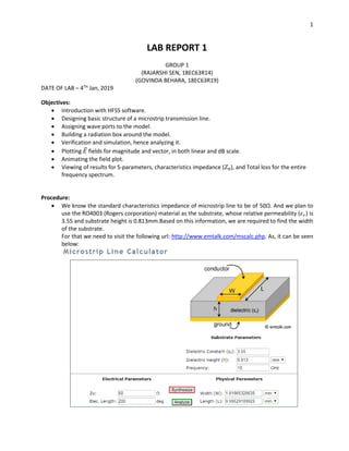
1. 1
LAB REPORT 1
GROUP 1
(RAJARSHI SEN, 18EC63R14)
(GOVINDA BEHARA, 18EC63R19)
DATE OF LAB – 4TH
Jan, 2019
Objectives:
• Introduction with HFSS software.
• Designing basic structure of a microstrip transmission line.
• Assigning wave ports to the model.
• Building a radiation box around the model.
• Verification and simulation, hence analyzing it.
• Plotting 𝐸⃗ fields for magnitude and vector, in both linear and dB scale.
• Animating the field plot.
• Viewing of results for S-parameters, characteristics impedance (𝑍0), and Total loss for the entire
frequency spectrum.
Procedure:
• We know the standard characteristics impedance of microstrip line to be of 50Ω. And we plan to
use the RO4003 (Rogers corporation) material as the substrate, whose relative permeability (𝜖 𝑟) is
3.55 and substrate height is 0.813mm.Based on this information, we are required to find the width
of the substrate.
For that we need to visit the following url: http://www.emtalk.com/mscalc.php. As, it can be seen
below:
2. 2
• There, all the values are put up. Frequency was taken as 10GHz, and the electrical length is of not
much importance, as its contribution to the width calculation is minimal. Then we get the
synthesized value of the width to be 1.81865mm. The second synthesized parameter, the Length
is again of less importance to us, so we ignored it.
• To start our design, we are needed to open up the HFSS software, which looks like:
• At first we designed the substrate, and for that we are needed to plot an arbitrary 3d box . The
reference grid is XY plane. To design the 3d box, two approaches can be taken:
o Drawing through the shortcut button: If we look carefully at the top, we will see a 3d
box icon which looks like:
Clicking it, will let us draw the 3d box.
o Alternatively, we can take up the original procedure of going through Draw > box. It
can be seen below:
3. 3
• Once we do that, then we get the markings on the grid that assists in drawing up the 3d box:
• Once, we are satisfied with the arbitrary box, we finalized it and the selected structure built
up:
• Next, we are required to change the box dimensions, so that we can make it up as the
substrate and it was suggested that we keep the origin of the space at the center of the
bottom of the substrate. We assumed the dimensions of the substrate to be the variables a,b
and h such that a=20mm, b=40mm and h=0.813mm(h was known earlier as the property of
RO4003c material). Variables assignment is deemed advantageous over direct values, as it
gives the flexibility to change the model dimensions without changing the physical structure
altogether.
The box that we created was arbitrarily named box1 and we can see it in the left side tab:
4. 4
• Then the following operations are performed:
Right click on “CreateBox” > Properties
• In HFSS, while defining the position, we need to refer to the starting position. So, for our
model of the substrate of dimension (a,b,h), the starting position would be (-a/2,-b/2 and 0)
and the size would be X axis – a, Y axis – b and Z axis – h. These valued have to be entered at
the following pop up window. It can be seen below:
5. 5
Following the variables declaration and position assignment, there opens successive popup for
variables definition, as seen above.
• Following that, we could see the final substrate dimension shaped up:
• Next, we changed the property of the substrate from vacuum to RO4003C and also changed
the name of the material for convenience. The procedure for it is:
Right click on “Box1” > Properties
6. 6
• In the popup window, we changed the name, and from the materials tab, we get the edit
options, where we searched for the desired material (RO4003C). The color of the substrate
was also changed to brown.
7. 7
• The ground plane is of same dimension as that of the substrate in x and y axis. The only
difference arises in the material type (copper) and thickness. So, the substrate was selected
and copied (selecting the substrate then ctrl + c and ctrl +v). A new material under RO4003C
named substrate1 was made.
• Following procedure is undertaken:
Right click on substrate 1 > Properties
• The material was edited from the tab and copper was selected. Also name was changed and
the color was changed to saffron.
• Then to change the physical location of the ground plane:
Right click on CreateBox > properties
8. 8
• The starting location of the ground plane is same as that of the substrate (-a/2,-b/2,0), and the
size of the ground plane a,b,-t. the thickness t is taken as negative (-t) because the thickness of
the ground plane will exist from Z=0 to z= -t. The thickness of the ground sheet was selected
as 17𝜇𝑚 (0.017mm).
• Then we visually verified the formation of ground plane below the substrate.
9. 9
• Next task was designing the microstrip. As its width was different from that of the substrate
and ground sheet, it was simpler to design the microstrip from beginning. For that we created
an arbitrary 3d box as before and then edited the physical dimension. The starting location of
the microstrip was –w/2,-b/2,h and the region was –w/2<X<w/2, -b/2<Y<b/2 and h<Z<h+t.
Then the size was X = w, Y = b and z = t. It was observed that the t is taken positive as the z
region starts from h and grows upward toward h+t. The width was earlier calculated to be
1.81865mm.
10. 10
• The name of the microstrip was changed from Box1 to “microstrip”, material changed to
copper and color changed to saffron.
• The finalized model was visible:
11. 11
• Next task was assigning of wave ports. For that we first changed the grid reference plane from
XY to XZ plane. First we searched for an icon resembling the following figure:
Then we get the dropdown menu and we select the desired plane.
• The change of grid plane was visible
• The ports are drawn as rectangular figures. For this again two approaches could have been
followed:
o Searching for the rectangular figure icon and selecting it. It looked like below:
o Draw > Rectangle
• Its physical starting dimensions are -3*w,-b/2,-t. It is known that the optimized value of the
wave port is six times the width of microstrip and 6 times the height of the substrate. It is
defined as below:
12. 12
• This was copied to form the next wave port and physical starting location was altered by
changing starting y location from –b/2 to b/2:
• The wave ports are visualized.
• Next we assigned wave port to the rectangular box that was just drawn. For that:
Right click on Rectangle1 > Assign Excitation > Wave port
14. 14
• Then an integration line was drawn:
• While drawing the line, we would get triangle symbols when cursor is at the exact center:
• If the previous procedure was done correctly, then it would show that the line was defined:
15. 15
• We can see that one of the sheets are classified as wave port:
• Then, similarly we will define the other sheet as wave port. After that, we can see that both
the sheets are under the category of wave port.
16. 16
• The next task was to verify the excitation of the wave port. For that, under the project
manager tab, we need to click on the excitation and then the respective port.
• Then we can see some regular geometry over the wave port, confirming the excitation
17. 17
• Next we were tasked with the design of a radiation box cover the microstrip transmission line.
For that, again, arbitrarily a 3d box was designed and, its material was selected as vacuum and
given the name of Rad_Box, also, color was set to light blue and transparency value was set to
0.9, allowing us to see the contents inside the radiation box.
• Then the physical dimensions were to be set. Generally the dimensions are such that, the
radiation box exceeds the substrate by the length of 𝜆0/4. In our case, it was a simple model,
so for convenience, we took the radiation box dimension as (a+20mm,b,h+20mm), and the
starting position was ((-a/2)-10mm,-b/2,0mm-10mm).
18. 18
• We could visualize the radiation box, and also the contents inside due to the assigned
transparency.
• Then, we have to assign the property of the radiation boundary to the radiation box. For that
Right click on Rad_Box > Assign Boundary > Radiation
19. 19
• The name was left as Rad1
• Then, to check for the boundary assignment we can click on the boundary option on the left
hand pane and then select Rad1.
20. 20
• Then we can view the regular geometry over the radiation box and be satisfied with the
boundary application.
• The radiation box was made invisible. For that, we open the active view visibility, and for that
we look for the icon with eye shape as given below:
Then, clicking it will open up the checkbox list for all the objects. We uncheck the Rad_Box.
21. 21
• The next step came for the simulation of the arrangement. For that we were needed to add a
solution setup.
Right click on Analysis > Add Solution Setup
• In the following popup window, the solution setup was set to 10GHz, as it is an broadband
structure, so center frequency was selected as the Solution Frequency (In narrowband
structures, the upper frequency is generally set as the solution frequency). The numbers of
passes (number of iterations) are selected as 20 (this parameter depends upon the processing
capability of the device).
22. 22
• Then, we defined the frequency sweep
Right click on Setup1 > Add Frequency Sweep
• The sweep type was selected as Fast sweep.
• Start frequency and stop frequency were taken up as 5GHz and 15GHz respectively. Step size
was selected as 0.02.
23. 23
• Then we need to verify the validity of the model. For this we looked up for a green icon
resembling a tick symbol as shown below.
• Clicking it shows whether all is done properly or otherwise.
• Once validation is verified, simulation had to begin. For this again another green icon next to
the previous one, resembling exclamation sign was clicked, which looked like the following:
• Following that, another popup opened up for saving the project and we named it as
“Microstrip report”.
24. 24
• Then simulation began, and we understood by some red progressive bars in the bottom right
corner
• Once the simulation ends, we will get the notification and also the red bars will not be there.
• We checked the fields on the wave port, by selecting Port field display, then 1 and then Port 1.
• Then appeared the field view.
25. 25
• We were interested in the region consisting of the microstrip, so we zoomed over to it.
The red arrows are strongest in the domain of magnitude. This result was reasonable.
• Next we checked the S-parameters, for this we needed to open the rectangular plot window
Right click on Results > Create Modal Solution Data Report > Rectangular Plot
26. 26
• From the following window, S Parameters were selected from the drop down menu. Both the
S(1,1) and S(2,1) were selected and the scale selected was dB.
• The S(2,1) should ideally be 1 in linear scale and 0 in dB, and S(1,1) should ideally be 0 in linear
scale and -∞ dB (in practical scenario, it would be some large negative value). The results we
obtained were:
27. 27
• We checked the magnitude of Electric field
Right click on substrate > Plot fields > E > Mag_E
• Frequency was selected as 10GHz and solution type was selected as sweep
28. 28
• To view the field, field overlays was selected, then E field and finally Mag_E1.
• We could see the plot of the radiation fields within the substrate.
29. 29
• The fields were concentrated mostly on the center. To see it more clearly, it was desired to
view this in log scale. For this we right clicked on the plot scale and selected the option
“Modify”.
• Then, in the following window, under the “scale” tab log was selected.
30. 30
• We could then see the fields more spread out, due to the log scale view.
• Next we went for the Vector electric fields.
Right click on substrate > Plot fields > E > Vector_E
31. 31
• Following the popup, again we selected the frequency to be 10Hz.
• We could visualize the Vector Electric fields.
32. 32
• We then performed the animation of the radiation over the substrate.
Right click on Mag_E1 > Animate
• Swept variable was kept as “Phase”
The animation was then visible.
33. 33
• As we went by the standard characteristics impedance of 50Ω, next we verified the port
impedance.
Right click on Results > Create Modal Solution Data Report > Rectangular Plot
• In the following window under the port Zo category, both Zo(1) and Zo(2) were selected and
scale was selected as Magnitude.
34. 34
• The characteristics impedance (𝑍0) for both the ports under entire frequency range was
visible.
• Then we checked the total loss through port 1. The following steps were taken:
Right click on Results > Create Modal Solution Data Report > Rectangular Plot
35. 35
• As the total loss is not a predefined variable, so we were needed to define it. From the popup
window, “output variables” is clicked upon.
• We know the total loss for port1 can be given as:
𝑇𝑜𝑡𝑎𝑙 𝐿𝑜𝑠𝑠 = 1 − |𝑆(1,1)|2
− |𝑆(2,1)|2
This equation was then written upon the expression space and added
• We had to confirm the addition of this new variable.
36. 36
• We followed through, selecting the new output variable we created
• We could see the plot representing total loss for entire frequency range.
Results:
• We gained familiarity with HFSS software.
• We successfully designed and tested the microstrip transmission line.
• The objectives were fulfilled.