The document outlines a practical manual for an Advanced Digital Signal Processing Lab at the University BDT College of Engineering, detailing experiments including the generation of discrete time signals, DFT and IDFT calculations, and PSD estimation using various methods. It also provides MATLAB scripts for signal generation, manipulation, and analysis, covering topics like DTMF signal generation, interpolation, and decimation of sequences. Additionally, it includes methods for time-frequency analysis and signal reconstruction using wavelet transforms.

1. 1
Dr. T.D. Shashikala Associate Professor Department of E&CE. University BDT College of
Engineering
UNIVERSITY BDT COLLEGE OF ENGINEERING. DAVANGERE-577004
(A constituent college of VISWESVARAYA TECHNOLOGICAL UNIVERSITY –
BELAGAVI)
Advanced Digital Signal Processing Lab Manuel 22LDN12
CIE for the PRACTICAL COMPONENT OF IPCC: 20(15+5) Marks
Prepared by
Dr. T.D. Shashikala
Associate Professor Department of E&CE
University BDT College of Engineering
( A Constituent College VTU Belagavi)
Davanagere – 577004
2021-22,
UPDATED 2024

2. 2
Dr. T.D. Shashikala Associate Professor Department of E&CE. University BDT College of
Engineering
Experiments mentioned in Syllabus
1 Generate various fundamental discrete time signals
2 Basic operations on signals (Multiplication, Folding, Scaling).
3 Find out the DFT & IDFT of a given sequence without using inbuilt
instructions.
4 Interpolation & decimation of a given sequence.
5 Generation of DTMF (Dual Tone Multiple Frequency) signals
6 Estimate the PSD of a noisy signal using periodogram and modified
periodogram
7 Estimation of PSD using different methods (Bartlett, Welch, Blackman-Tukey).
8 Design of Chebyshev Type I, II Filters.
9 Cascade Digital IIR Filter Realization.
10 Parallel Realization of IIR filter.
11 Estimation of power spectrum using parametric methods (YuleWalker
&Burg).
12 Time-Frequency Analysis with the Continuous Wavelet Transform.
13 Signal Reconstruction from Continuous Wavelet Transform Coefficients.

3. 3
Dr. T.D. Shashikala Associate Professor Department of E&CE. University BDT College of
Engineering
1. Generate various fundamental discrete time signals
a) impulse: for varying amplitudes and time duration
b) step signal: at t=0, t<0 and t>0 with varying amplitudes
c) ramp signal; positive and negative ramp signals of varying slopes
d) exponential signal: increasing and decreasing exponential within limited
time period
e) sinusoidal signal: varying amplitudes and frequencies
clc;close all;clear all;
% a) Impulse signal
amplitude = 5;
duration = 5;
t_impulse = -duration:1:duration;
x_impulse = zeros(size(t_impulse));
x_impulse(duration + 1) = amplitude;
figure;
stem(t_impulse, x_impulse, 'LineWidth', 2);
xlabel('Time');
ylabel('Amplitude');
title('Impulse Signal');
% b) Step signal
amplitude_step = 3;
t_step = -10:1:10;
x_step = amplitude_step * (t_step >= 0);
figure;
stem(t_step, x_step, 'LineWidth', 2);
xlabel('Time');
ylabel('Amplitude');
title('Step Signal');
% c) Ramp signal
slope = 2;
t_ramp = -10:1:10;
x_ramp = slope * t_ramp;
figure;
stem(t_ramp, x_ramp, 'LineWidth', 2);
xlabel('Time');
ylabel('Amplitude');

4. 4
Dr. T.D. Shashikala Associate Professor Department of E&CE. University BDT College of
Engineering
title('Ramp Signal');
% d) Exponential signal
amplitude_exp = 2;
duration_exp = 5;
t_exp = -duration_exp:1:duration_exp;
x_exp_increase = amplitude_exp * exp(t_exp);
x_exp_decrease = amplitude_exp * exp(-t_exp);
figure;
stem(t_exp, x_exp_increase, 'LineWidth', 2);
xlabel('Time');
ylabel('Amplitude');
title('Increasing Exponential Signal');
figure;
stem(t_exp, x_exp_decrease, 'LineWidth', 2);
xlabel('Time');
ylabel('Amplitude');
title('Decreasing Exponential Signal');
% e) Sinusoidal signal
amplitude_sine = 3;
frequency = 1;
t_sine = 0:0.01:10;
x_sine = amplitude_sine * sin(2*pi*frequency*t_sine);
figure;
plot(t_sine, x_sine, 'LineWidth', 2);
xlabel('Time');
ylabel('Amplitude');
title('Sinusoidal Signal');
OUTPUT
This script will generate the same signals as before, but without using functions. Each
section corresponds to one of the signal types, and it directly generates the signals and plots
them without encapsulating them into functions.

5. 5
Dr. T.D. Shashikala Associate Professor Department of E&CE. University BDT College of
Engineering

6. 6
Dr. T.D. Shashikala Associate Professor Department of E&CE. University BDT College of
Engineering
2 Basic operations on signals (Multiplication, Folding, Scaling)
clc;close all;clear all;
% Define the original signal
t = -5:0.1:5;
x = exp(-t); % Exponential signal
% Plot the original signal
subplot(3, 2, 1);
plot(t, x, 'LineWidth', 2);
xlabel('Time');
ylabel('Amplitude');
title('Original Signal');
% a) Multiplication of the signal with a constant
k = 2; % Constant value
x_mult = k * x; % Multiplication operation
% Plot the multiplied signal
subplot(3, 2, 2);
plot(t, x_mult, 'LineWidth', 2);
xlabel('Time');
ylabel('Amplitude');
title('Multiplied Signal (k * x)');
% b) Folding of the signal
t_fold = -fliplr(t); % Time reversal
x_fold = fliplr(x); % Signal reversal
% Plot the folded signal
subplot(3, 2, 3);
plot(t_fold, x_fold, 'LineWidth', 2);
xlabel('Time');
ylabel('Amplitude');
title('Folded Signal');
% c) Scaling of the signal
a = 0.5; % Scaling factor
t_scale = a * t; % Time scaling
x_scale = x; % Amplitude remains unchanged
% Plot the scaled signal

7. 7
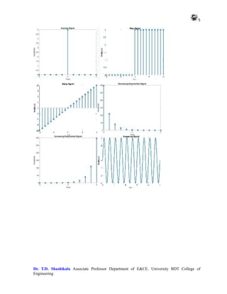
Dr. T.D. Shashikala Associate Professor Department of E&CE. University BDT College of
Engineering
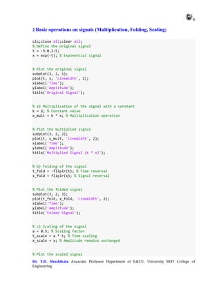
subplot(3, 2, 4);
plot(t_scale, x_scale, 'LineWidth', 2);
xlabel('Time');
ylabel('Amplitude');
title('Scaled Signal (a * t)');
% d) Combined operations: Multiplication, Folding, and Scaling
x_combined = k * fliplr(a * x); % Multiplication, folding, and scaling
% Plot the combined signal
subplot(3, 2, [5, 6]);
plot(t_fold, x_combined, 'LineWidth', 2);
xlabel('Time');
ylabel('Amplitude');
title('Combined Operation (k * x(-at))');
OUTPUT
This script performs the same operations as before, including multiplication with a constant,
folding, scaling, and a combination of these operations, without using functions. Each
operation is illustrated in a separate subplot

8. 8
Dr. T.D. Shashikala Associate Professor Department of E&CE. University BDT College of
Engineering

9. 9
Dr. T.D. Shashikala Associate Professor Department of E&CE. University BDT College of
Engineering
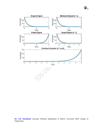
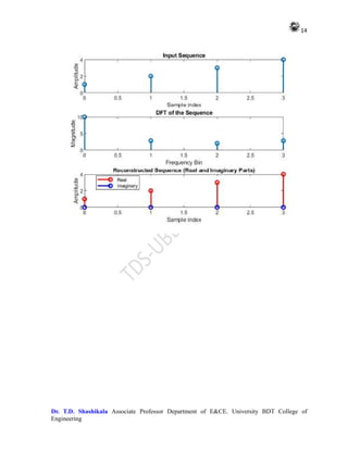
3. Find out the DFT and IDFT of a given sequence without using inbuilt
instructions
clc;clear all;close all;
% Define the sequence
x = [1, 2, 3, 4]; % Example sequence
% DFT Calculation
N = length(x);
X = zeros(1, N);
for k = 1:N
for n = 1:N
X(k) = X(k) + x(n) * exp(-1i*2*pi*(k-1)*(n-1)/N);
end
end
% IDFT Calculation
x_reconstructed = zeros(1, N);
for n = 1:N
for k = 1:N
x_reconstructed(n) = x_reconstructed(n) + (1/N) * X(k) *
exp(1i*2*pi*(k-1)*(n-1)/N);
end
end
% Display results
disp('DFT:');
disp(X);
disp('IDFT:');
disp(x_reconstructed);
OUTPUT
In this code:
x is the input sequence.
N is the length of the sequence.
X is the DFT of the sequence x.
x_reconstructed is the reconstructed sequence after applying the IDFT.
You can replace the example sequence x with any sequence you want to
compute the DFT and IDFT for.

10. 10
Dr. T.D. Shashikala Associate Professor Department of E&CE. University BDT College of
Engineering
Make sure to understand the mathematical formulas behind the DFT and IDFT
algorithms to implement them correctly.
DFT:
10.0000 + 0.0000i -2.0000 + 2.0000i -2.0000 - 0.0000i -2.0000 -
2.0000i
IDFT:
1.0000 - 0.0000i 2.0000 - 0.0000i 3.0000 - 0.0000i 4.0000 +
0.0000i
Alternate Method
% Define the sequence
x = [1, 2, 3, 4]; % Example sequence
% DFT Calculation
N = length(x);
X = zeros(1, N);
for k = 1:N
for n = 1:N
X(k) = X(k) + x(n) * exp(-1i*2*pi*(k-1)*(n-1)/N);
end
end
% Plotting
subplot(2, 1, 1);
stem(0:N-1, x, 'LineWidth', 2);
xlabel('Sample index');
ylabel('Amplitude');
title('Input Sequence');
subplot(2, 1, 2);
stem(0:N-1, abs(X), 'LineWidth', 2);
xlabel('Frequency Bin');
ylabel('Magnitude');
title('DFT of the Sequence');
OUTPUT 2

11. 11
Dr. T.D. Shashikala Associate Professor Department of E&CE. University BDT College of
Engineering

12. 12
Dr. T.D. Shashikala Associate Professor Department of E&CE. University BDT College of
Engineering
ALTERNATE METHOD
clc; close all; clear all;
% Define the sequence
x = [1, 2, 3, 4]; % Example sequence
% DFT Calculation
N = length(x);
X = zeros(1, N);
for k = 1:N
for n = 1:N
X(k) = X(k) + x(n) * exp(-1i*2*pi*(k-1)*(n-1)/N);
end
end
% IDFT Calculation
x_reconstructed = zeros(1, N);
for n = 1:N
for k = 1:N
x_reconstructed(n) = x_reconstructed(n) + (1/N) * X(k) *
exp(1i*2*pi*(k-1)*(n-1)/N);
end
end

13. 13
Dr. T.D. Shashikala Associate Professor Department of E&CE. University BDT College of
Engineering
% Plotting
subplot(3, 1, 1);
stem(0:N-1, x, 'LineWidth', 2);
xlabel('Sample index');
ylabel('Amplitude');
title('Input Sequence');
subplot(3, 1, 2);
stem(0:N-1, abs(X), 'LineWidth', 2);
xlabel('Frequency Bin');
ylabel('Magnitude');
title('DFT of the Sequence');
subplot(3, 1, 3);
stem(0:N-1, real(x_reconstructed), 'r', 'LineWidth', 2);
hold on;
stem(0:N-1, imag(x_reconstructed), 'b', 'LineWidth', 2);
xlabel('Sample index');
ylabel('Amplitude');
title('Reconstructed Sequence (Real and Imaginary Parts)');
legend('Real', 'Imaginary', 'Location', 'Best');
OUTPUT
This code computes the DFT and IDFT of the given sequence x, and plots the input
sequence, its DFT (magnitude), and the real and imaginary parts of the reconstructed
sequence (after applying IDFT). Each plot has appropriate labels and titles. You can
run this code in MATLAB to see the plots.

14. 14
Dr. T.D. Shashikala Associate Professor Department of E&CE. University BDT College of
Engineering

15. 15
Dr. T.D. Shashikala Associate Professor Department of E&CE. University BDT College of
Engineering
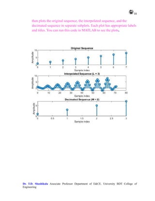
4. Interpolation & decimation of a given sequence
clc; close all; clear all;
% Define the original sequence
x = [1, 2, 3, 4, 5, 6, 7, 8]; % Example sequence
% Interpolation
L = 3; % Interpolation factor
x_interp = zeros(1, length(x) * L);
x_interp(1:L:end) = x; % Insert zeros in between
x_interp = interp(x_interp, L); % Interpolation using built-in interp
function
% Decimation
M = 2; % Decimation factor
x_decimated = x(1:M:end); % Select every Mth sample
% Plotting
subplot(3, 1, 1);
stem(0:length(x)-1, x, 'LineWidth', 2);
xlabel('Sample index');
ylabel('Amplitude');
title('Original Sequence');
subplot(3, 1, 2);
stem(0:length(x_interp)-1, x_interp, 'LineWidth', 2);
xlabel('Sample index');
ylabel('Amplitude');
title('Interpolated Sequence (L = 3)');
subplot(3, 1, 3);
stem(0:length(x_decimated)-1, x_decimated, 'LineWidth', 2);
xlabel('Sample index');
ylabel('Amplitude');
title('Decimated Sequence (M = 2)');
OUTPUT
This MATLAB program defines an original sequence x, performs
interpolation with a factor L of 3, and decimation with a factor M of 2. It

16. 16
Dr. T.D. Shashikala Associate Professor Department of E&CE. University BDT College of
Engineering
then plots the original sequence, the interpolated sequence, and the
decimated sequence in separate subplots. Each plot has appropriate labels
and titles. You can run this code in MATLAB to see the plots.

17. 17
Dr. T.D. Shashikala Associate Professor Department of E&CE. University BDT College of
Engineering
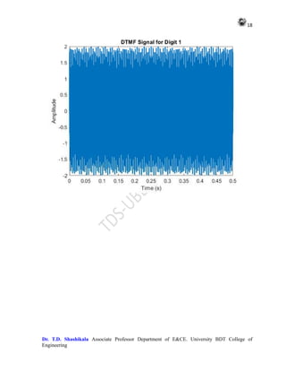
5. Generation of DTMF (Dual Tone Multiple Frequency) signals
clc; close all;clear all;
% Define the digit for which DTMF signal will be generated
digit = 1; % Example digit
% Define the frequencies corresponding to each DTMF digit
dtmf_freqs = [697, 770, 852, 941; % Row frequencies
1209, 1336, 1477, 1633]; % Column frequencies
% Define the time axis
fs = 8000; % Sampling frequency
duration = 0.5; % Duration of each tone in seconds
t = 0:1/fs:duration;
% Generate DTMF signal for the input digit
row_idx = ceil(digit/4); % Row index
col_idx = mod(digit-1, 4) + 1; % Column index
tone1 = sin(2*pi*dtmf_freqs(1, row_idx)*t); % Row tone
tone2 = sin(2*pi*dtmf_freqs(2, col_idx)*t); % Column tone
dtmf_signal = tone1 + tone2; % Combined DTMF signal
% Plot the DTMF signal
figure;
plot(t, dtmf_signal, 'LineWidth', 2);
xlabel('Time (s)');
ylabel('Amplitude');
title(['DTMF Signal for Digit ', num2str(digit)]);
OUTPUT
This code generates a DTMF signal for the specified digit, plots it, and displays the
corresponding DTMF signal. You can change the value of digit to generate DTMF signals for
different digits. Adjust the sampling frequency, duration, and other parameters as needed.

18. 18
Dr. T.D. Shashikala Associate Professor Department of E&CE. University BDT College of
Engineering

19. 19
Dr. T.D. Shashikala Associate Professor Department of E&CE. University BDT College of
Engineering
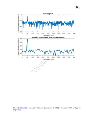
6. Estimate the PSD of a noisy signal using periodogram and modified
periodogram
% Generate a noisy signal
fs = 1000; % Sampling frequency
t = 0:1/fs:1-1/fs; % Time vector
x = cos(2*pi*50*t) + randn(size(t)); % Noisy signal with sinusoidal component
% Compute the periodogram
[Pxx, f] = periodogram(x, [], [], fs);
% Compute the modified periodogram with Bartlett window
[Pxx_bartlett, f_bartlett] = pwelch(x, [], [], [], fs);
% Plot the PSD estimates
figure;
subplot(2, 1, 1);
plot(f, 10*log10(Pxx), 'LineWidth', 2);
xlabel('Frequency (Hz)');
ylabel('Power/Frequency (dB/Hz)');
title('Periodogram');
subplot(2, 1, 2);
plot(f_bartlett, 10*log10(Pxx_bartlett), 'LineWidth', 2);
xlabel('Frequency (Hz)');
ylabel('Power/Frequency (dB/Hz)');
title('Modified Periodogram with Bartlett Window');
OUTPUT
In this code:
We generate a noisy signal x containing a sinusoidal component and add Gaussian
noise to it.
We then compute the periodogram using the periodogram function and the modified
periodogram with Bartlett window using the pwelch function.
Finally, we plot the PSD estimates obtained from both methods.
You can adjust the parameters such as the sampling frequency, signal frequency, and
noise characteristics according to your requirements.

20. 20
Dr. T.D. Shashikala Associate Professor Department of E&CE. University BDT College of
Engineering

21. 21
Dr. T.D. Shashikala Associate Professor Department of E&CE. University BDT College of
Engineering
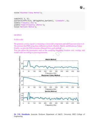
7 Estimation of PSD using different methods (Bartlett, Welch, Blackman-
Tukey).
% Generate a noisy signal
fs = 1000; % Sampling frequency
t = 0:1/fs:1-1/fs; % Time vector
x = cos(2*pi*50*t) + randn(size(t)); % Noisy signal with sinusoidal component
% Define parameters
N = length(x); % Length of the signal
M = 100; % Window size for Bartlett and Welch methods
overlap = 50; % Overlap for Welch method
nfft = 2^nextpow2(N); % FFT length for Welch method
% Bartlett method
n_segments = floor(N / M); % Number of segments
Pxx_bartlett = zeros(nfft/2 + 1, 1); % Initialize PSD
for i = 1:n_segments
segment = x((i-1)*M+1 : i*M); % Extract segment
Pxx_bartlett = Pxx_bartlett + periodogram(segment, [], nfft, fs) /
n_segments; % Compute periodogram
end
% Welch method
[Pxx_welch, f_welch] = pwelch(x, hamming(M), overlap, nfft, fs); % Compute
Welch PSD
% Blackman-Tukey method
[Pxx_bt, f_bt] = pburg(x, 4, nfft, fs); % Compute Blackman-Tukey PSD
% Plot the PSD estimates
figure;
subplot(3, 1, 1);
plot(f_welch, 10*log10(Pxx_welch), 'LineWidth', 2);
xlabel('Frequency (Hz)');
ylabel('Power/Frequency (dB/Hz)');
title('Welch Method');
subplot(3, 1, 2);
plot(f_bt, 10*log10(Pxx_bt), 'LineWidth', 2);
xlabel('Frequency (Hz)');
ylabel('Power/Frequency (dB/Hz)');

22. 22
Dr. T.D. Shashikala Associate Professor Department of E&CE. University BDT College of
Engineering
title('Blackman-Tukey Method');
subplot(3, 1, 3);
plot(0:fs/nfft:fs/2, 10*log10(Pxx_bartlett), 'LineWidth', 2);
xlabel('Frequency (Hz)');
ylabel('Power/Frequency (dB/Hz)');
title('Bartlett Method');
OUTPUT
In this code:
We generate a noisy signal x containing a sinusoidal component and add Gaussian noise to it.
We estimate the PSD using three different methods: Bartlett, Welch, and Blackman-Tukey.
Finally, we plot the PSD estimates obtained from each method.
You can adjust the parameters such as the sampling frequency, window size, overlap, and
model order according to your requirements

23. 23
Dr. T.D. Shashikala Associate Professor Department of E&CE. University BDT College of
Engineering
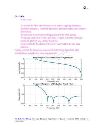
8. Design of Chebyshev Type I, II Filters
% Define filter specifications
fs = 1000; % Sampling frequency
fpass = 100; % Passband frequency (Hz)
fstop = 200; % Stopband frequency (Hz)
ripple_pass = 0.5; % Passband ripple (dB)
ripple_stop = 60; % Stopband attenuation (dB)
% Normalized frequencies
Wp = fpass / (fs/2);
Ws = fstop / (fs/2);
% Design Chebyshev Type I filter
[N1, Wn1] = cheb1ord(Wp, Ws, ripple_pass, ripple_stop);
[b1, a1] = cheby1(N1, ripple_pass, Wn1);
% Design Chebyshev Type II filter
[N2, Wn2] = cheb2ord(Wp, Ws, ripple_pass, ripple_stop);
[b2, a2] = cheby2(N2, ripple_stop, Wn2);
% Frequency response
[h1, w1] = freqz(b1, a1, 512, fs);
[h2, w2] = freqz(b2, a2, 512, fs);
% Plot frequency response of Chebyshev Type I filter
figure;
subplot(2, 1, 1);
plot(w1, 20*log10(abs(h1)), 'LineWidth', 2);
xlabel('Frequency (Hz)');
ylabel('Magnitude (dB)');
title('Frequency Response of Chebyshev Type I Filter');
grid on;
% Plot frequency response of Chebyshev Type II filter
subplot(2, 1, 2);
plot(w2, 20*log10(abs(h2)), 'LineWidth', 2);
xlabel('Frequency (Hz)');
ylabel('Magnitude (dB)');
title('Frequency Response of Chebyshev Type II Filter');
grid on;

24. 24
Dr. T.D. Shashikala Associate Professor Department of E&CE. University BDT College of
Engineering
OUTPUT
In this code:
We define the filter specifications such as the sampling frequency,
passband frequency, stopband frequency, passband ripple, and stopband
attenuation.
We calculate the normalized frequencies for the filter design.
We design Chebyshev Type I and Type II filters using the cheb1ord,
cheb2ord, cheby1, and cheby2 functions.
We compute the frequency response of each filter using the freqz
function.
Finally, we plot the frequency response of both filters. Adjust the filter
specifications according to your requirements.

25. 25
Dr. T.D. Shashikala Associate Professor Department of E&CE. University BDT College of
Engineering
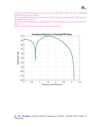
9. Cascade Digital IIR Filter Realization
% Define the coefficients of the individual filters
b1 = [0.1, 0.2, 0.1];
a1 = [1, -0.5, 0.2];
b2 = [0.2, -0.3, 0.2];
a2 = [1, 0.1, 0.3];
% Generate the frequency response of the first filter
[H1, W1] = freqz(b1, a1);
% Generate the frequency response of the second filter
[H2, W2] = freqz(b2, a2);
% Zero-pad the frequency responses to have the same length
N = max(length(H1), length(H2));
H1 = padarray(H1, [0, N - length(H1)], 'post');
H2 = padarray(H2, [0, N - length(H2)], 'post');
% Cascade the filters by element-wise multiplication
H_cascade = H1 .* H2;
% Plot the frequency response of the cascaded filter
figure;
plot(W1, 20*log10(abs(H_cascade)), 'LineWidth', 2);
xlabel('Frequency (rad/sample)');
ylabel('Magnitude (dB)');
title('Frequency Response of Cascaded IIR Filters');
grid on;
OUTPUT
In this code:
We define the coefficients b1, a1 for the numerator and denominator polynomials of the first
filter.
We define the coefficients b2, a2 for the numerator and denominator polynomials of the second
filter.
We use the freqz function to compute the frequency response of each filter.
We cascade the filters by convolving their frequency responses.

26. 26
Dr. T.D. Shashikala Associate Professor Department of E&CE. University BDT College of
Engineering
Finally, we plot the frequency response of the cascaded filter. Adjust the filter coefficients
according to your requirements.
We use the padarray function to zero-pad the shorter frequency response (H1 or H2) to match
the length of the longer one.
We then perform element-wise multiplication (.*) of the frequency responses to cascade the
filters.
Finally, we plot the frequency response of the cascaded filter.

27. 27
Dr. T.D. Shashikala Associate Professor Department of E&CE. University BDT College of
Engineering
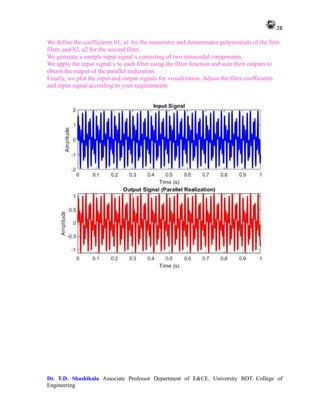
10. Parallele Realization of IIR Filter
% Define the coefficients of the IIR filters
b1 = [0.1, 0.2, 0.1];
a1 = [1, -0.5, 0.2];
b2 = [0.2, -0.3, 0.2];
a2 = [1, 0.1, 0.3];
% Generate a sample input signal
fs = 1000; % Sampling frequency
t = 0:1/fs:1-1/fs; % Time vector
x = sin(2*pi*50*t) + sin(2*pi*120*t); % Input signal
% Apply the input signal to each filter and sum their outputs
y1 = filter(b1, a1, x);
y2 = filter(b2, a2, x);
y_parallel = y1 + y2;
% Plot the input and output signals
figure;
subplot(2, 1, 1);
plot(t, x, 'b', 'LineWidth', 2);
xlabel('Time (s)');
ylabel('Amplitude');
title('Input Signal');
grid on;
subplot(2, 1, 2);
plot(t, y_parallel, 'r', 'LineWidth', 2);
xlabel('Time (s)');
ylabel('Amplitude');
title('Output Signal (Parallel Realization)');
grid on;
OUTPUT
In this code:

28. 28
Dr. T.D. Shashikala Associate Professor Department of E&CE. University BDT College of
Engineering
We define the coefficients b1, a1 for the numerator and denominator polynomials of the first
filter, and b2, a2 for the second filter.
We generate a sample input signal x consisting of two sinusoidal components.
We apply the input signal x to each filter using the filter function and sum their outputs to
obtain the output of the parallel realization.
Finally, we plot the input and output signals for visualization. Adjust the filter coefficients
and input signal according to your requirements.

29. 29
Dr. T.D. Shashikala Associate Professor Department of E&CE. University BDT College of
Engineering
11. Estimation of Power spectrum using parametric methods (Yule-Walker
& Burg)
clc; close all;clear all;
% Generate a noisy signal
fs = 1000; % Sampling frequency
t = 0:1/fs:1-1/fs; % Time vector
x = cos(2*pi*50*t) + randn(size(t)); % Noisy signal with sinusoidal component
% Model order
p = 4;
% Yule-Walker method using Levinson-Durbin recursion
[rxx, lags] = xcorr(x, p, 'biased'); % Estimate autocorrelation
r = rxx(p+2:end); % Autocorrelation vector
a_yw = levinson(r, p); % Estimate AR coefficients
% Burg method
[a_burg, e_burg, k_burg] = pburg(x, p, p, fs); % Estimate AR coefficients
% Compute power spectrum using Yule-Walker method
[H_yw, w_yw] = freqz(1, a_yw, 512, fs);
% Compute power spectrum using Burg method
[H_burg, w_burg] = freqz(1, a_burg, 512, fs);
% Plot the power spectrum estimates
figure;
subplot(2, 1, 1);
plot(w_yw, 20*log10(abs(H_yw)), 'LineWidth', 2);
xlabel('Frequency (Hz)');
ylabel('Power/Frequency (dB/Hz)');
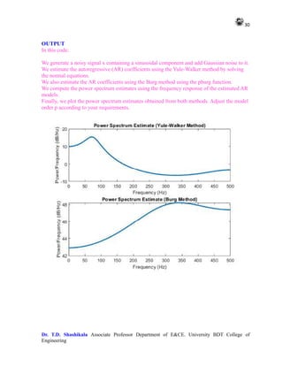
title('Power Spectrum Estimate (Yule-Walker Method)');
subplot(2, 1, 2);
plot(w_burg, 20*log10(abs(H_burg)), 'LineWidth', 2);
xlabel('Frequency (Hz)');
ylabel('Power/Frequency (dB/Hz)');
title('Power Spectrum Estimate (Burg Method)');

30. 30
Dr. T.D. Shashikala Associate Professor Department of E&CE. University BDT College of
Engineering
OUTPUT
In this code:
We generate a noisy signal x containing a sinusoidal component and add Gaussian noise to it.
We estimate the autoregressive (AR) coefficients using the Yule-Walker method by solving
the normal equations.
We also estimate the AR coefficients using the Burg method using the pburg function.
We compute the power spectrum estimates using the frequency response of the estimated AR
models.
Finally, we plot the power spectrum estimates obtained from both methods. Adjust the model
order p according to your requirements.

31. 31
Dr. T.D. Shashikala Associate Professor Department of E&CE. University BDT College of
Engineering
13. Time Frequency Analysis with the continuous wavelet Transform
clc; close all;clear all;
% Define the signal
fs = 1000; % Sampling frequency
t = 0:1/fs:1-1/fs; % Time vector
f0 = 50; % Frequency of the signal
x = cos(2*pi*f0*t); % Signal with frequency 50 Hz
% Define Morlet wavelet function inline
morlet = @(scale, fs) exp(2*pi*1i*5*(-scale/2:1/fs:scale/2)) .* exp(-
(scale/(2*pi))^2*(-scale/2:1/fs:scale/2).^2);
% Define wavelet parameters
scales = 1:128; % Wavelet scales
frequencies = scal2frq(scales, 'morl', 1/fs); % Corresponding frequencies
% Perform Continuous Wavelet Transform (CWT)
cwt_result = zeros(length(scales), length(t)); % Initialize CWT result matrix
for i = 1:length(scales)
scale = scales(i);
wavelet = morlet(scale, fs); % Generate Morlet wavelet
cwt_result(i, :) = conv(x, wavelet, 'same'); % Perform convolution
end
% Plot the Time-Frequency Representation
figure;
imagesc(t, frequencies, abs(cwt_result));
colormap('jet');
colorbar;
xlabel('Time (s)');
ylabel('Frequency (Hz)');
title('Time-Frequency Representation using Continuous Wavelet Transform');
Output:
In this code:
We define a simple sinusoidal signal x with a frequency of 50 Hz.
We define the wavelet scales and corresponding frequencies.

32. 32
Dr. T.D. Shashikala Associate Professor Department of E&CE. University BDT College of
Engineering
We loop through each scale, generate the Morlet wavelet, and perform convolution with the
input signal to obtain the CWT coefficients.
Finally, we plot the time-frequency representation using the obtained CWT coefficients.
Note: This is a basic implementation. For more efficient and advanced CWT algorithms,
consider using built-in functions like cwt in MATLAB.

33. 33
Dr. T.D. Shashikala Associate Professor Department of E&CE. University BDT College of
Engineering
12. Design of LPC filter using Levinson-Durbin Algorithm
% Define the input signal
x = randn(1, 1000); % Random input signal of length 1000
% Order of the LPC filter
p = 10;
% Calculate autocorrelation of input signal
R = xcorr(x, p, 'biased');
% Implement the Levinson-Durbin recursion
[a, e] = levinson(R, p);
% Display the filter coefficients
disp('Filter coefficients:');
disp(a);
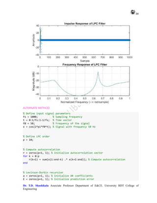
% Plot the impulse response of the LPC filter
impulse_response = filter([0 -a(2:end)], 1, [1 zeros(1, length(x)-1)]);
figure;
subplot(2,1,1);
stem(impulse_response);
title('Impulse Response of LPC Filter');
xlabel('Sample');
ylabel('Amplitude');
% Plot the frequency response of the LPC filter
[h, w] = freqz(1, a, 1024);
subplot(2,1,2);
plot(w/pi, 20*log10(abs(h)));
title('Frequency Response of LPC Filter');
xlabel('Normalized Frequency (timespi rad/sample)');
ylabel('Magnitude (dB)');
grid on;
This code generates a random input signal, calculates its autocorrelation, applies the
Levinson-Durbin recursion to estimate the LPC coefficients, and then plots the impulse
response and frequency response of the resulting LPC filter. You can adjust the order p of the
filter according to your requirements.

34. 34
Dr. T.D. Shashikala Associate Professor Department of E&CE. University BDT College of
Engineering
ALTERNATE METHOD
% Define input signal parameters
fs = 1000; % Sampling frequency
t = 0:1/fs:1-1/fs; % Time vector
f0 = 50; % Frequency of the signal
x = cos(2*pi*f0*t); % Signal with frequency 50 Hz
% Define LPC order
p = 10;
% Compute autocorrelation
r = zeros(p+1, 1); % Initialize autocorrelation vector
for k = 0:p
r(k+1) = sum(x(1:end-k) .* x(k+1:end)); % Compute autocorrelation
end
% Levinson-Durbin recursion
a = zeros(p+1, 1); % Initialize AR coefficients
E = zeros(p+1, 1); % Initialize prediction error

35. 35
Dr. T.D. Shashikala Associate Professor Department of E&CE. University BDT College of
Engineering
a(1) = 1; % First coefficient is always 1
for k = 1:p
% Compute k-th AR coefficient
num = r(k+1:-1:2).' * a(1:k); % Numerator of the recursion formula
den = r(1:k).' * a(1:k); % Denominator of the recursion formula
a(k+1) = -num / (den + eps);
% Update prediction error
E(k+1) = (1 - a(k+1)^2) * E(k);
% Update previous coefficients and error
a(1:k) = a(1:k) + a(k+1) * flipud(a(1:k));
end
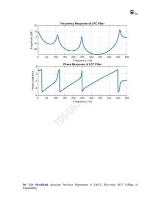
% Compute frequency response of LPC filter
[H, w] = freqz(1, a, 512, fs);
% Plot frequency response
figure;
subplot(2,1,1);
plot(w, 20*log10(abs(H)), 'LineWidth', 2);
xlabel('Frequency (Hz)');
ylabel('Magnitude (dB)');
title('Frequency Response of LPC Filter');
grid on;
subplot(2,1,2);
plot(w, angle(H), 'LineWidth', 2);
xlabel('Frequency (Hz)');
ylabel('Phase (radians)');
title('Phase Response of LPC Filter');
grid on;
This code estimates the autocorrelation of the input signal and computes the LPC coefficients
using the Levinson-Durbin recursion. It then plots the magnitude and phase response of the
LPC filter. Adjust the LPC order p according to your requirements. Let me know if you need
further explanation or assistance!

36. 36
Dr. T.D. Shashikala Associate Professor Department of E&CE. University BDT College of
Engineering

37. 37
Dr. T.D. Shashikala Associate Professor Department of E&CE. University BDT College of
Engineering
14. Signal Reconstruction from Continuous Wavelet Transform Co-efficient
We define a simple sinusoidal signal x and its time vector t.
We choose a wavelet (here, cmor, the Complex Morlet wavelet) and a range of scales
(here, 1 to 64) for the wavelet transform.
We compute the CWT coefficients using the cwt function.
We reconstruct the signal from the CWT coefficients using the icwt function.
Finally, we plot the original and reconstructed signals for comparison.
You can adjust the signal, wavelet, scales, and other parameters according to your specific
needs.
% Define the signal and its parameters
t = linspace(0, 1, 1000); % Time vector
f0 = 10; % Frequency of the signal
x = sin(2*pi*f0*t); % Original signal
% Define the wavelet and its parameters
wavelet = 'morl'; % Complex Morlet wavelet
scales = 1:64; % Range of scales for the wavelet
% Calculate the corresponding frequencies for the scales
frequencies = scal2frq(scales, wavelet, 1); % Corresponding frequencies
% Calculate the continuous wavelet transform
coefficients = cwt(x, scales, wavelet);
% Reconstruct the signal from the coefficients
reconstructed_signal = icwt(coefficients, scales, wavelet, 'FreqRange', frequencies,
'SamplingPeriod', mean(diff(t)));
% Plot original and reconstructed signals
figure;
subplot(2,1,1);
plot(t, x);
title('Original Signal');
xlabel('Time');
ylabel('Amplitude');
subplot(2,1,2);
plot(t, reconstructed_signal);

38. 38
Dr. T.D. Shashikala Associate Professor Department of E&CE. University BDT College of
Engineering
title('Reconstructed Signal');
xlabel('Time');
ylabel('Amplitude');