Download as PDF, PPTX


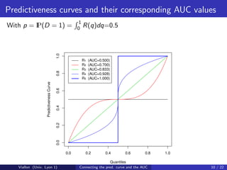
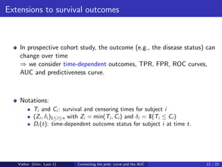
![Predictiveness curve for binary outcomes
Many alternative criteria have been proposed for evaluating
discrimination
proportion of explained variation,
standardized total gain
risk reclassification measures (Pencina et al., SiM, 2006)
Most of them express as simple functions of the predictiveness curve
(Gu and Pepe, Int. J. Biostatistics, 2009).
Denote by G −1 the quantile function of X . For any q ∈ [0, 1], let
R(q) = P D = 1|X = G −1 (q)
be the risk associated to the qth quantile of X .
The predictiveness curve plots R(q) versus q.
Viallon (Univ. Lyon 1) Connecting the pred. curve and the AUC 9 / 22](https://image.slidesharecdn.com/aucsilverspring-111027075118-phpapp02/85/Auc-silver-spring-9-320.jpg)
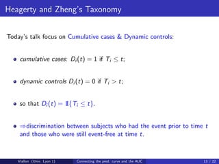
![The relation in the binary outcome setting
Still denote by R the predictiveness curve of marker X ,
R(q) = P D = 1|X = G −1 (q) .
1
Then, denoting by p = IP(D = 1) = 0 R(q)dq the disease
prevalence, the AUC of marker X is given by
1
0 qR(q)dq − p 2 /2
AUC =
p(1 − p)
We can check that
AUC = 0.5 when R(q) = p;
AUC = 1 when R(q) = 1 [1−p,1] (q).
I
Viallon (Univ. Lyon 1) Connecting the pred. curve and the AUC 11 / 22](https://image.slidesharecdn.com/aucsilverspring-111027075118-phpapp02/85/Auc-silver-spring-11-320.jpg)
![Workaround for AUCC,D
Using Bayes’s theorem (see, e.g., Chambless & Diao)
∞ ∞
F (t0 ; X = x)[1 − F (t0 ; X = c)]
AUCC,D (t0 ) = g (x)g (c)dxdc
−∞ c [1 − F (t0 )]F (t0 )
with
P(T ≤ t) be the risk function at time t;
F (t) = I
P(T ≤ t|X = x) be the conditional risk function at
F (t; X = x) = I
time t;
g the density function of marker X .
Viallon (Univ. Lyon 1) Connecting the pred. curve and the AUC 15 / 22](https://image.slidesharecdn.com/aucsilverspring-111027075118-phpapp02/85/Auc-silver-spring-16-320.jpg)
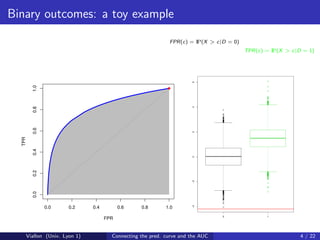
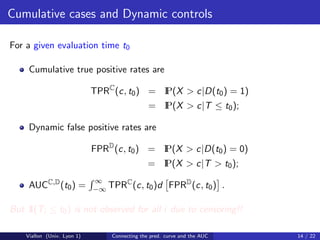
![Predictiveness curve and AUCC,D
Introduce
P(D(t) = 1|X = G −1 (q))
R(t; q) := I
= P(T ≤ t|X = G −1 (q))
I
the time-dependent predictiveness curve
We established that
1 2
C,D 0 qR(t0 ; q)dq − F (t0 )
2
AUC (t0 ) =
F (t0 )[1 − F (t0 )]
Proper estimation of R(t0 ; q) (especially for q 1) should yield
proper estimation of AUCC,D (t0 )
Viallon (Univ. Lyon 1) Connecting the pred. curve and the AUC 16 / 22](https://image.slidesharecdn.com/aucsilverspring-111027075118-phpapp02/85/Auc-silver-spring-17-320.jpg)
![Sketch of the proof
∞ ∞
F (t; X = x)[1 − F (t; X = c)]g (x)g (c)dxdc
−∞ c
1 1
−1 −1
= F (t; X = G (u))[1 − F (t; X = G (v ))]dudv
0 v
1 1
−1 −1
= [1 − S(t; X = G (u))]S(t; X = G (v ))dudv
0 v
1 1 1
−1 −1 −1
= (1 − v )S(t; X = G (v ))dv − S(t; X = G (u))S(t; X = G (v ))dudv
0 0 v
1 1 1
−1 −1 −1
= (1 − v )S(t; X = G (v ))dv − S(t; X = G (u))S(t; X = G (v ))1I(u ≥ v )dudv .
0 0 0
Setting
−1 −1
L(u, v ) = S(t; X = G (u))S(t; X = G (v )),
we have L(u, v ) = L(v , u) so that
∞ ∞
F (t; X = x)[1 − F (t; X = c)]g (x)g (c)dxdc
−∞ c
1 1 1 1
−1 −1 −1
= (1 − v )S(t; X = G (v ))dv − S(t; X = G (u))S(t; X = G (v ))dudv
0 2 0 0
1 1 1 2
−1 −1
= (1 − v )S(t; X = G (v ))dv − S(t; X = G (v ))dv .
0 2 0](https://image.slidesharecdn.com/aucsilverspring-111027075118-phpapp02/85/Auc-silver-spring-24-320.jpg)
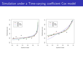

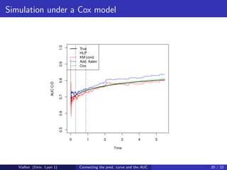
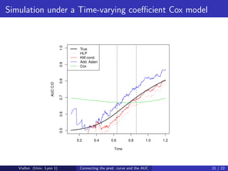
This document discusses methods for evaluating discrimination for survival outcomes using time-dependent measures. It connects the time-dependent area under the ROC curve (AUC) to the time-dependent predictiveness curve. The AUC can be estimated based on the predictiveness curve, which plots the risk of an event versus quantiles of a marker over time. Simulation studies assess the impact of model misspecification when estimating the conditional risk function used to derive estimates of the time-dependent AUC.