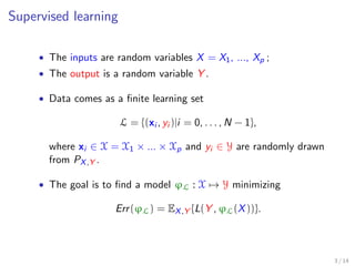
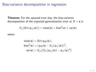
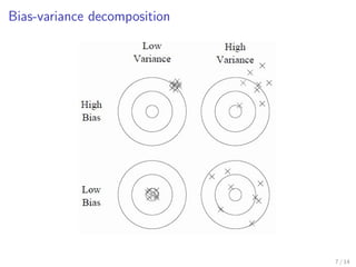
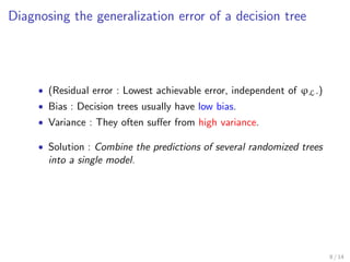
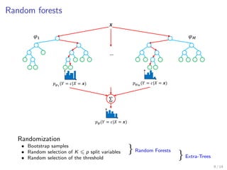
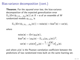
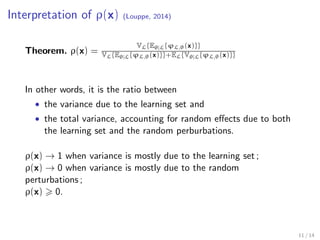
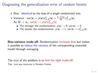
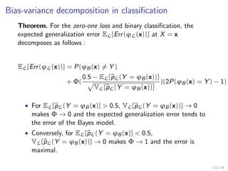
This document discusses bias-variance decomposition in random forests. It explains that combining predictions from multiple randomized models can achieve better results than a single model by reducing variance. Random forests work by constructing decision trees on randomly selected subsets of data and features, averaging their predictions. This randomization increases bias but reduces variance, providing an effective bias-variance tradeoff. The document provides theorems on how the expected generalization error of random forests and individual trees can be decomposed into noise, bias, and variance components.

1. Bias-variance decomposition
in Random Forests
Gilles Louppe @glouppe
Paris ML S02E04, December 8, 2014
1 / 14

2. Motivation
In supervised learning, combining the predictions of several
randomized models often achieves better results than a single
non-randomized model.
Why ?
2 / 14

3. Supervised learning
The inputs are random variables X = X1, ..., Xp ;
The output is a random variable Y .
Data comes as a

4. nite learning set
L = f(xi , yi )ji = 0, . . . ,N - 1g,
where xi 2 X = X1 ... Xp and yi 2 Y are randomly drawn
from PX,Y .
The goal is to

5. nd a model 'L : X7! Y minimizing
Err ('L) = EX,Y fL(Y ,'L(X))g.
3 / 14

6. Performance evaluation
Classi

7. cation
Symbolic output (e.g., Y = fyes, nog)
Zero-one loss
L(Y ,'L(X)) = 1(Y6= 'L(X))
Regression
Numerical output (e.g., Y = R)
Squared error loss
L(Y ,'L(X)) = (Y - 'L(X))2
4 / 14

8. Decision trees
0.7
0.5
X1
X2
t5 t3 t4
푡2
푡1
푋1 ≤ 0.7
푡3
푡4 푡5
풙
푝(푌 = 푐|푋 = 풙)
Split node
≤ Leaf node
푋2 ≤ 0.5 ≤
t 2 ' : nodes of the tree '
Xt : split variable at t
vt 2 R : split threshold at t
'(x) = arg maxc2Y p(Y = cjX = x)
5 / 14

9. Bias-variance decomposition in regression
Theorem. For the squared error loss, the bias-variance
decomposition of the expected generalization error at X = x is
ELfErr ('L(x))g = noise(x) + bias2(x) + var(x)
where
noise(x) = Err ('B(x)),
bias2(x) = ('B(x) - ELf'L(x)g)2,
var(x) = ELf(ELf'L(x)g - 'L(x))2g.
6 / 14

10. Bias-variance decomposition
7 / 14

11. Diagnosing the generalization error of a decision tree
(Residual error : Lowest achievable error, independent of 'L.)
Bias : Decision trees usually have low bias.
Variance : They often suer from high variance.
Solution : Combine the predictions of several randomized trees
into a single model.
8 / 14

12. Random forests
풙
휑1 휑푀
푝휑1 (푌 = 푐|푋 = 풙)
…
푝휑푚 (푌 = 푐|푋 = 풙)
Σ
푝휓(푌 = 푐|푋 = 풙)
Randomization
Bootstrap samples Random selection of K 6 p split variables g Random Forests Random selection of the threshold g Extra-Trees
9 / 14

13. Bias-variance decomposition (cont.)
Theorem. For the squared error loss, the bias-variance
decomposition of the expected generalization error
ELfErr ( L,1,...,M (x))g at X = x of an ensemble of M
randomized models 'L,m is
ELfErr ( L,1,...,M (x))g = noise(x) + bias2(x) + var(x),
where
noise(x) = Err ('B(x)),
bias2(x) = ('B(x) - EL,f'L,(x)g)2,
var(x) = (x)2
L,(x) +
1 - (x)
M
2
L,(x).
and where (x) is the Pearson correlation coecient between the
predictions of two randomized trees built on the same learning set.
10 / 14

14. Interpretation of (x) (Louppe, 2014)
Theorem. (x) =
VLfEjLf'L,(x)gg
VLfEjLf'L,(x)gg+ELfVjLf'L,(x)gg
In other words, it is the ratio between
the variance due to the learning set and
the total variance, accounting for random eects due to both
the learning set and the random perburbations.
(x) ! 1 when variance is mostly due to the learning set ;
(x) ! 0 when variance is mostly due to the random
perturbations ;
(x) 0.
11 / 14