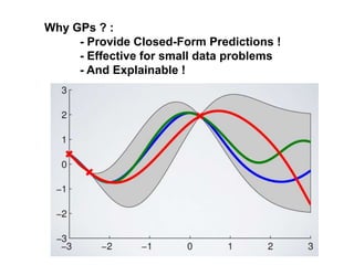
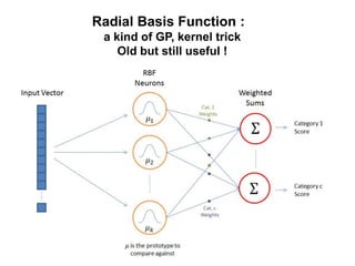
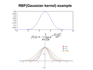
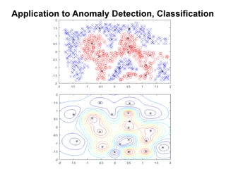
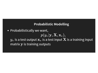
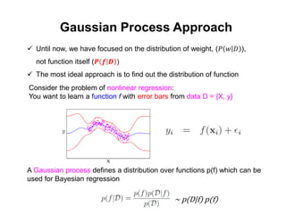
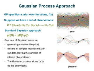
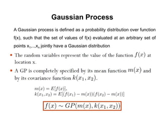
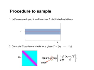
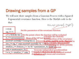
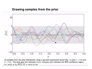
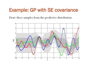
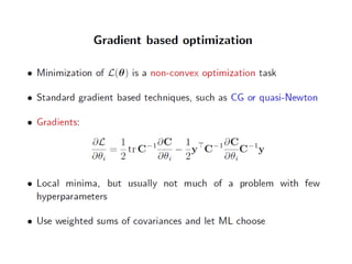
Gaussian Processes
Regression, Classification & Optimization
2019. 1. 23
김 홍 배
Why GPs ? :
- Provide Closed-Form Predictions !
- Effective for small data problems
- And Explainable !
Radial Basis Function :
a kind of GP, kernel trick
Old but still useful !
RBF(Gaussian kernel) example
Application to Anomaly Detection, Classification
Optimal Data Sampling Strategy !
Difficult to tangle !
How Do We Deal With Many Parameters, Little Data ?
1. Regularization
e.g., smoothing, L1 penalty, drop out in neural nets, large K
for K-nearest neighbor
2. Standard Bayesian approach
specify probability of data given weights, P(D|W)
specify weight priors given hyper-parameter α, P(W|α)
find posterior over weights given data, P(W|D, α)
With little data, strong weight prior constrains inference
3. Gaussian processes
place a prior over functions, p(f) directly rather than
over model parameters, p(w)
Functions : Relationship between Input and Output
Distribution of functions that satisfy
within the range of Input, X and Output, f
 Prior over functions, No Constraints
X
f
prior
Gaussian Process Approach
 Until now, we have focused on the distribution of weight, (𝑃 𝑤 𝐷 ),
not function itself (𝑷 𝒇 𝑫 )
 The most ideal approach is to find out the distribution of function
Consider the problem of nonlinear regression:
You want to learn a function f with error bars from data D = {X, y}
A Gaussian process defines a distribution over functions p(f) which can be
used for Bayesian regression
~ p(D|f) p(f)
 GP specifies a prior over functions, f(x)
 Suppose we have a set of observations:
D = {(x1,y1), (x2, y2), (x3, y3), …, (xn, yn)}
Standard Bayesian approach
p(f|D) ~ p(D|f) p(f)
One view of Bayesian inference
• generating samples (the prior)
• discard all samples inconsistent with
our data, leaving the samples of
interest (the posterior)
• The Gaussian process allows us to
do this analytically.
Gaussian Process Approach
prior
posterior
 Bayesian data modeling technique that account for uncertainty
 Bayesian kernel regression machines
Gaussian Process Approach
Gaussian Process
A Gaussian process is defined as a probability distribution over function
f(x), such that the set of values of f(x) evaluated at an arbitrary set of
points x1,..,xn jointly have a Gaussian distribution
Two input vectors are close  There outputs are highly correlated
Two input vectors are far away  There outputs are uncorrelated
If (x-x’) ~ 0  k(x,x’) ~ v
If (x-x’) ∞  k(x,x’)  0
Distance bw. inputs
Prior Distribution of Function
Sampling from the prior distribution of a GP at arbitrary points, X*
𝑓𝑝𝑟𝑖 𝑥∗ ~𝐺𝑃 𝑚 𝑥∗ , 𝐾(𝑥∗, 𝑥∗)
𝑓𝑝𝑟𝑖 𝑥∗ ~𝐺𝑃 0, 𝐾(𝑥∗, 𝑥∗)
Without loss of generality, assume 𝑚 𝑥 = 0, Var(𝐾(𝑥∗, 𝑥∗)) =1
Function depends only on the Covariance !!
Procedure to sample
2. Compute Covariance Matrix for a given 𝑋 = 𝑥1 … . 𝑥 𝑛
1. Let’s assume input, X and function, f distributed as follows
X
f
Procedure to sample
3. Compute SVD or Cholesky decomp. of K to get orthogonal basis
functions
K = 𝐴𝑆𝐵 𝑇 = 𝐿𝐿𝑇
4. Compute Basis Function
𝑓𝑖 = 𝐴𝑆1/2 𝑢𝑖
or 𝑓𝑖 = 𝐿𝑢𝑖
𝑢𝑖 ∶ 𝑟𝑎𝑛𝑑𝑜𝑚 𝑣𝑒𝑐𝑡𝑜𝑟 𝑤𝑖𝑡ℎ
𝑧𝑒𝑟𝑜 𝑚𝑒𝑎𝑛 𝑎𝑛𝑑 𝑢𝑛𝑖𝑡 𝑣𝑎𝑟𝑖𝑎𝑛𝑐𝑒
L : Lower part of Cholesky
decomp. of K
X
f
posterior
X
f
prior
Set the parameters of the covariance function
Set the points where the function will be evaluated
Mean of the GP (set to zero)
Generate all the possible pairs of points
Calculate the covariance
function for all the possible
pairs of points
Calculate the Cholesky
decomposition of the covariance
function (add 10-9 to the diagonal to
ensure positive definiteness).
Generate independent pseudorandom
numbers drawn from the standard normal
distribution.
Compute f which has the desired
distribution with mean and covariance
Drawing samples from the prior
NxN matrix N*xN matrix NxN* matrix N*xN*
4 observations (training points)
Calculate the partitions of
the joint covariance matrix
Cholesky decomposition of
K(X,X) – training of GP
Complexity O(N3)
Calculate predictive
distribution
ComplexityO(N2)
Testing points range from -10 ~ 10
Samples from the posterior pass close to the observations, but vary a lot in
regions where are no observations.
Standard deviation of the noise on the observation
Add the noise to the diagonal of K(X,X)
Gaussian processing
Gaussian processing
Gaussian processing
Gaussian processing
Gaussian processing
Gaussian processing
Gaussian processing
Gaussian processing

Gaussian processing

  • 1.
    Gaussian Processes Regression, Classification& Optimization 2019. 1. 23 김 홍 배
  • 2.
    Why GPs ?: - Provide Closed-Form Predictions ! - Effective for small data problems - And Explainable !
  • 3.
    Radial Basis Function: a kind of GP, kernel trick Old but still useful !
  • 4.
  • 5.
    Application to AnomalyDetection, Classification
  • 6.
  • 10.
  • 11.
    How Do WeDeal With Many Parameters, Little Data ? 1. Regularization e.g., smoothing, L1 penalty, drop out in neural nets, large K for K-nearest neighbor 2. Standard Bayesian approach specify probability of data given weights, P(D|W) specify weight priors given hyper-parameter α, P(W|α) find posterior over weights given data, P(W|D, α) With little data, strong weight prior constrains inference 3. Gaussian processes place a prior over functions, p(f) directly rather than over model parameters, p(w)
  • 12.
    Functions : Relationshipbetween Input and Output Distribution of functions that satisfy within the range of Input, X and Output, f  Prior over functions, No Constraints X f prior
  • 13.
    Gaussian Process Approach Until now, we have focused on the distribution of weight, (𝑃 𝑤 𝐷 ), not function itself (𝑷 𝒇 𝑫 )  The most ideal approach is to find out the distribution of function Consider the problem of nonlinear regression: You want to learn a function f with error bars from data D = {X, y} A Gaussian process defines a distribution over functions p(f) which can be used for Bayesian regression ~ p(D|f) p(f)
  • 14.
     GP specifiesa prior over functions, f(x)  Suppose we have a set of observations: D = {(x1,y1), (x2, y2), (x3, y3), …, (xn, yn)} Standard Bayesian approach p(f|D) ~ p(D|f) p(f) One view of Bayesian inference • generating samples (the prior) • discard all samples inconsistent with our data, leaving the samples of interest (the posterior) • The Gaussian process allows us to do this analytically. Gaussian Process Approach prior posterior
  • 15.
     Bayesian datamodeling technique that account for uncertainty  Bayesian kernel regression machines Gaussian Process Approach
  • 16.
    Gaussian Process A Gaussianprocess is defined as a probability distribution over function f(x), such that the set of values of f(x) evaluated at an arbitrary set of points x1,..,xn jointly have a Gaussian distribution
  • 17.
    Two input vectorsare close  There outputs are highly correlated Two input vectors are far away  There outputs are uncorrelated
  • 19.
    If (x-x’) ~0  k(x,x’) ~ v If (x-x’) ∞  k(x,x’)  0 Distance bw. inputs
  • 20.
    Prior Distribution ofFunction Sampling from the prior distribution of a GP at arbitrary points, X* 𝑓𝑝𝑟𝑖 𝑥∗ ~𝐺𝑃 𝑚 𝑥∗ , 𝐾(𝑥∗, 𝑥∗) 𝑓𝑝𝑟𝑖 𝑥∗ ~𝐺𝑃 0, 𝐾(𝑥∗, 𝑥∗) Without loss of generality, assume 𝑚 𝑥 = 0, Var(𝐾(𝑥∗, 𝑥∗)) =1 Function depends only on the Covariance !!
  • 21.
    Procedure to sample 2.Compute Covariance Matrix for a given 𝑋 = 𝑥1 … . 𝑥 𝑛 1. Let’s assume input, X and function, f distributed as follows X f
  • 22.
    Procedure to sample 3.Compute SVD or Cholesky decomp. of K to get orthogonal basis functions K = 𝐴𝑆𝐵 𝑇 = 𝐿𝐿𝑇 4. Compute Basis Function 𝑓𝑖 = 𝐴𝑆1/2 𝑢𝑖 or 𝑓𝑖 = 𝐿𝑢𝑖 𝑢𝑖 ∶ 𝑟𝑎𝑛𝑑𝑜𝑚 𝑣𝑒𝑐𝑡𝑜𝑟 𝑤𝑖𝑡ℎ 𝑧𝑒𝑟𝑜 𝑚𝑒𝑎𝑛 𝑎𝑛𝑑 𝑢𝑛𝑖𝑡 𝑣𝑎𝑟𝑖𝑎𝑛𝑐𝑒 L : Lower part of Cholesky decomp. of K X f posterior X f prior
  • 23.
    Set the parametersof the covariance function Set the points where the function will be evaluated Mean of the GP (set to zero) Generate all the possible pairs of points Calculate the covariance function for all the possible pairs of points Calculate the Cholesky decomposition of the covariance function (add 10-9 to the diagonal to ensure positive definiteness). Generate independent pseudorandom numbers drawn from the standard normal distribution. Compute f which has the desired distribution with mean and covariance
  • 24.
  • 25.
    NxN matrix N*xNmatrix NxN* matrix N*xN*
  • 28.
    4 observations (trainingpoints) Calculate the partitions of the joint covariance matrix Cholesky decomposition of K(X,X) – training of GP Complexity O(N3) Calculate predictive distribution ComplexityO(N2) Testing points range from -10 ~ 10
  • 30.
    Samples from theposterior pass close to the observations, but vary a lot in regions where are no observations.
  • 35.
    Standard deviation ofthe noise on the observation Add the noise to the diagonal of K(X,X)