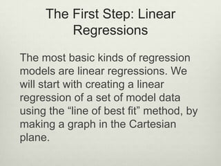
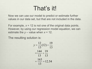
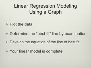
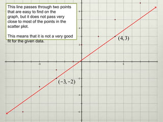
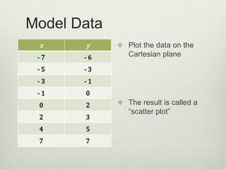
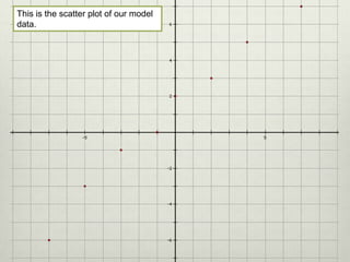
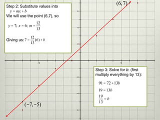
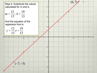
1) Regression models analyze data to find patterns and relationships that can be used to predict future trends or values. 2) A linear regression finds the line of best fit to model the relationship between two variables in a data set. 3) The document demonstrates how to create a linear regression model by plotting sample data, determining the best fit line, calculating the line's slope and y-intercept, and writing the equation in slope-intercept form.

1. Linear
Regression
Modeling
Using a Graph & the Line of Best Fit

2. What is a regression model?
Many times in an For example, if we are
given the equation
algebra problem we
2
are given an y= x+6 ,
3
equation, and
we can then calculate y
asked to calculate given different values of x.
values using that
equation. So if x = 3 , then y = 8
and if x = 6 , then y = 10

3. What is a regression model?
But sometimes, we are given the data
and asked to create an equation that
models the data.
In other words, we already have the
answers but need to figure out the
equation that gives us those answers.

4. What is a regression model?
In mathematics, this is called a
regression model, since we are sort
of working backwards to find an
equation, when we already have the
answers.

5. Why do we need them?
Regression models have many
applications in industry and science.
 Regression models can predict future
trends, like population growth.
 Regression models can be used to estimate
costs and profits for businesses.
 Regression models can help medical care
professionals determine how much medication
to prescribe for their patients.

6. The First Step: Linear
Regressions
The most basic kinds of regression
models are linear regressions. We
will start with creating a linear
regression of a set of model data
using the “line of best fit” method, by
making a graph in the Cartesian
plane.

7. Linear Regression Modeling
Using a Graph
 Plot the data
 Determine the “best fit” line by examination
 Develop the equation of the line of best fit
 Your linear model is complete

8. Model Data
x y  Plot the data on the
-7 -6 Cartesian plane
-5 -3
-3 -1
-1 0
0 2  The result is called a
“scatter plot”
2 3
4 5
7 7

9. This is the scatter plot of our model
data.

10. Adding the best fit line
1. The best fit line should:
a) Pass through two points that are easy to find on the
graph.
b) Come as close as possible to as many of the data
points in the scatter plot as possible
2. There should be about the same number of points
from the scatter plot above the line as below it.
3. The best fit line can pass through some of the
points on the scatter plot, but it does not have to
pass through any of them.

11. This line does not pass through two
points that are easy to find on the
graph.
This will make it more difficult to
determine the equation of this line.

12. This line passes through two points
that are easy to find on the
graph, but it does not pass very
close to most of the points in the
scatter plot.
This means that it is not a very good
fit for the given data.
(4, 3)
(-3, -2)

13. This line passes close to many of the
data points in the scatter plot, but
most of the points are above the line; (6, 6)
only one point is below the line.
We’re getting closer!
(-3, -2)

14. The line passes through two easy to
(6, 7)
find points.
It passes close to most of the points
in the scatter plot.
There are several points both above
and below the line.
This looks like a good fit for the data!
Remember, there may be
more than one line that is a
good fit. You have to decide
which one looks “best” to
you.
(-7, -5)

15. Find the Equation of Your Best-fit
Line
1. Calculate the slope of the line
2. Using the slope-intercept form of a linear equation,
y = mx + b , substitute one of the points on your
best-fit line into the equation for x and y, and
substitute the slope you found in step 1.
3. Solve the resulting equation for b, giving you the y-
intercept.
4. Rewrite the equation in slope-intercept form using
the correct values for slope and the y-intercept (b).

16. Step 1: Calculate slope
(6, 7)
The slope of this line is:
(-7, -5)

17. Step 2: Substitute values into
(6, 7)
y = mx + b
We will use the point (6,7), so
12
y = 7; x = 6; m =
13
12
Giving us: 7 = (6) + b
13
Step 3: Solve for b: (first
multiply everything by 13):
91 = 72 +13b
19 = 13b
19
=b
13
(-7, -5)

18. (6, 7)
Step 4: Substitute the values
calculated for m and b.
12 19
m= ; b=
13 13
And the equation of the
regression line is:
12 19
y= x+
13 13
(-7, -5)

19. That’s it!
Now we can use our model to predict or estimate further
values in our data set, but that are not included in the data.
For example, x = 12 is not one of the original data points.
However, by using our regression model equation, we can
estimate the y – value when x = 12.
The resulting solution is:
12 19
y= (12) +
13 13
144 19
= +
13 13
163
= = 12.54
13