This document discusses using a graph dynamical system to model the vertex coloring problem. It proposes using a Graph-cellular Automaton (GA), which is an extension of cellular automata, to distribute the coloring process. In the GA model, each vertex independently chooses its optimal color based on the colors of its adjacent vertices. The document outlines testing the GA approach on different types of graphs and analyzing whether it can find colorings for them. It provides background on graph coloring, planar graphs, and introduces the graph dynamical system and GA models.

1. GRAPH COLOURING ON GRAPH
DYNAMICAL SYSTEM
Clyde Shen
Supervisor by:
Dr. Jiamou Liu
November 21, 2013
1

2. Abstract
Vertex colouring problem is a combinatorial problem in which a colour
is assigned to each vertex of the graph such that no two adjacent ver-
tices have the same colour[6]. We initialize the use of graph dynamical
system to model a distributed computation for solving the vertex colour-
ing problem on graphs. Graph dynamical system provide a model of
Graph-cellular Automaton to find a way to colour graph. In this report
Graph-cellular Automaton is proposed for finding a solution of the ver-
tex colouring problem. Each vertex chooses its optimal colour based on
the colours selected by its adjacent vertices. A simulation experiments is
to show the proposed algorithm. The obtained results show whether the
graph dynamical system is appropriate for solving colouring problem.
Contents
1 Introduction 3
2 Planar Graph and Colouring 4
2.1 Planar Graph . . . . . . . . . . . . . . . . . . . . . . . . . . . . . 4
2.2 Graph Colouring . . . . . . . . . . . . . . . . . . . . . . . . . . . 7
3 Graph Dynamical System 8
3.1 basic problem . . . . . . . . . . . . . . . . . . . . . . . . . . . . . 8
4 Graph Colouring with GDS 10
4.1 implementation of colouring graph with GDS . . . . . . . . . . . 10
4.2 Colour some specified case . . . . . . . . . . . . . . . . . . . . . . 11
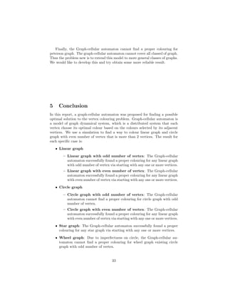
5 Conclusion 33
2

3. 1 Introduction
Graph colouring problem is a classical combinatorial optimization problem ni
graph theory. Graph colouring show up a great many kind of forms, for exam-
ple, vertex colouring, edge colouring, multicolouring, etc[1]. Graph colouring is
widely used in our life, such as computer register allocation[4], air traffic flow
management[2], and so on. Colouring is a well-known NP-hard problem for gen-
eral graph[9]. Vertex colouring problem is also a well-know colouring problem.
A proper vertex colouring of graph G = (V, E) where V is the set of |V | vertices
and E is the set of |E| edge, is to assign different colours to each vertex in order
that no two adjacent vertices are given the same colour. The chromatic number
χ(G) is a colouring parameter defined as the minimum number of colours that
should appear in the most colourful closed neighbourhood of a vertex under any
proper colouring of the graph[3].
Cellular automata are dynamical systems in computability theory, mathemat-
ics, etc, which were originally discovered by John von Neumann in 1940s[8].
The use of the Cellular Automata (CA) paradigm is emerging as a powerful
approach to the analysis and design of complex systems[10]. It is an important
model in computation theory. Cellular automata basically consists of a regular
grid of cells, each in one of a finite number of states, such as 0 or 1. CA has
self-organizing behaviour for every cell according to some fixed rule from their
neighbours[1]. Cellular automata also works on the vertex colouring problem
by using dynamical system[7]. Some model and distribute algorithm have been
used to solve the vertex colouring problem, such as Irregular cellular learning
automata[1], dynamic colouring[7], etc.
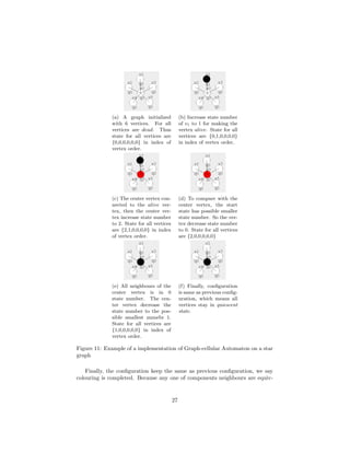
In this report, we initialize the use of graph dynamical system to model a agent-
based computation for solving the vertex colouring problem. In this system, a
input graph is run by an Graph-cellular Automaton (GA), which is an extended
cellular automata. To do this, a global transition is made up by local transitions
of each vertex. Each vertex is distributed and locally run at each independent
step. The proposed system is composed of a number of configurations, and the
each configuration of colouring is locally found for each vertex and its neigh-
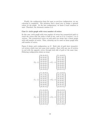
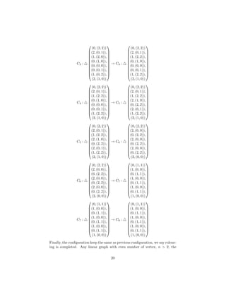
bours. Finally, if a configuration is same as previous configuration, we say the
system found a way to colour the graph. On the other hand, if a configuration
always is different from previous one and repeat varieties of configurations in
some way, we say the system is in a loop. Therefore, if the system found a
way to colour a graph, then the chromatic number of the graph is total size of
distinct state on the graph, otherwise we say the system might not find a good
way to colour the graph.
The structure of this report is as follows. In the next section, an overview
of the basic theory and proof on planar graph and colouring. Graph dynam-
ical system on graph colouring is introduced in Section 4. Also a model and
simulator of Graph-cellular automaton will be introduced in the second part
3

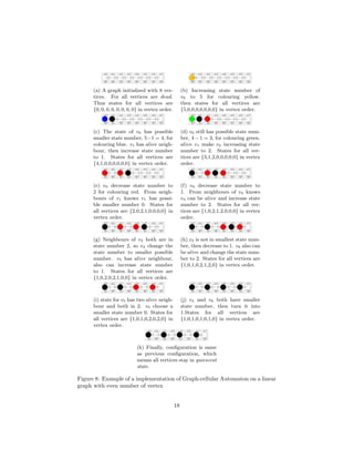
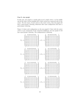
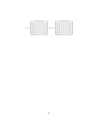
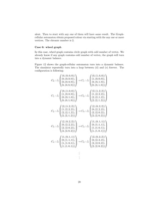
4. of Section 4. The simulator perform various case studies to solving the vertex
colouring problem using graph dynamical system, such as linear graph, circle
graph, star graph, wheel graph and Peterson graph. For each case we focus on
a specific class of graph and investigate the use of graph dynamical systems on
these graphs.
2 Planar Graph and Colouring
Colouring graph is central to graph theory. In this section we introduce the
basic definition and terminology on graph colouring.
2.1 Planar Graph
Definition 2.1. (Planar Graph) A planar graph is a graph that can be drawn
on a plane surface in such a way that on two edges of it intersect (except for
intersections in vertices)[5].
Example 2.2. The complete graph K4 consists 4 vertices and with an edge
between every pair of vertices is planar. Figure 1a shows a representation of
K4 in a plane, which does not prove K4 is planar. Figure 1b shows that K4 is
planar graph.
(a) The planar graph K4 draw
with two edges intersecting.
(b) The planar graph K4 draw
without two edges intersecting.
Figure 1: Example of a planar graphs
Definition 2.3. (Face) The faces of plane graph G = (V, E) is the regions of
R2
G, which are subsets of R. Hence G is bounded. For Example, G lies inside
some adequately large disc D; exactly one of its faces is unbounded, the face
4

5. that contains R2
D. The outer face of G is the unbounded; the other faces are
inner faces. Every (finite) planar graph has exactly one infinite face[5].
We denote the set of faces of G by F(G).
Theorem 2.4. (Euler’s Formula) If we use v to denote the number of ver-
tices of a graph, e to denote the number of edges, and f to denote the number
of faces[5]. A connected plane graph with v(≥ 1) vertices, e edges and f faces
then
v − e + f = 2.
Example 2.5. The figure 2 shows a connected planar graph K4 consisting v = 4
vertices, e = 6 edges and f = 4 faces, where the face a, b and c is inner faces,
and d is the infinite outer face. Thus we have v − e + f = 4 − 6 + 4 = 2
a
b
c
d
(a) In the planar graph K4, the face a, b
and c are inner faces; The face d is the in-
finite outer face.
Figure 2
Proof. Basis: Consider the case e = 0. In this case, v must be 1 since G is
connected. With 1 vertex and no edges, there is exactly one outer faces. Thus
v − e + f = 1 − 0 + 1 = 2 as desired. Inductive step. Assume that the statement
is true for any connected planar graph with at most k edges. In other words,
for any connected planar graph G = (V, E) with v vertices, e ≤ k edges, and r
faces, v − e + f = 2. This is the inductive hypothesis. Suppose G = (V, E) is a
connected planar graph with v vertices, e = k + 1 vertices, and f faces.
If G is a tree, then e = v − 1.In addition, If G is a tree,then the only one face is
the outer face surround the tree so f = 1. Thus v − e + f = v − (v − 1) + 1 = 2
as desired.
If G is not a tree, then G has some cycle, which we use C to denote the cycle. Let
e be any edge in C, and consider a subgraph G = (V, E {e}) of G. G must be
5

6. connected because removing an edge from a cycle breaks the cycle but does not
break the connectivity of the graph. Furthermore, G has one fewer face than G
because removing an edge merges two faces into one face. Because subgraph of
a planar graph is also planar and |E| = e = k+1, G is a connected planar graph
with |E {e}| = k edges. Thus the inductive hypothesis applies to G to yield
v−k+(f −1) = 2. Therefore, v−e+f = v−(k+1)+f = v−k+(f −1) = 2.
Lemma 2.6. If a connected planar graph G = (V, E) has more than 2 vertices,
|V | ≥ 2, then |E| ≤ 3|V | − 6.[3]
Proof. If the number of edges is less or equal to 3, |E| ≤ 3, and |V | > 2, then
the theorem can be verified directly.
Otherwise, because the number of edges is bigger than 3, every face is bounded
by at least 3 edges. In addition, every edge bounds at most 2 faces. Thus,
3|F| 2|E|, so |F| 2|E|
3 or r 2e
3 .
Apply the relation and substituting it into Euler’s formula[2.4], v − e + f = 2,
we get v − e + 2e
3 2. This implies that 3v − e 6 or |E| ≤ 3|V | − 6, and the
lemma is proved.
Theorem 2.7. The complete graph K5, is not a planar graph[5]
Figure 3: The non-planar graph K5
Proof. Suppose graph K5 is a planar graph. So, the graph K5 have |V | = 5
vertices, |E| = 10 edges. We know e 3v − 6 from Lemma[2.6]. So, if v = 5
then 3 × 5 − 6 = 9. However, 10 9, and the theory is proved.
Theorem 2.8. The complete bipartite graph with three vertices on each side,
K3,3 is not a planar graph [5]
Proof. Assume that K3,3 is planar graph. K3,3 has 6 vertices and 9 edges. Let
F be the set of faces in the planar representation of K3,3. By Euler’s Formula
2.4, we have |F| = 2 − |V | + |E| = 2 − 6 + 9 = 5.
Consider the set B = {(v, f) ∈ V × F|v is on the border of f}. We bound
6

7. Figure 4: The non-planar graph K3,3
its size in two different ways.
Every face has a cycle as its border. Note that the shortest this cycle can
be is 4. It cannot be 1 or 2 for the same reason as in the previous proof. More-
over, it cannot be 3 because K3,3 is bipartite. Every cycle begins and ends at
the same vertex, and edges go between vertices in two different halves of the
graph. Thus, after 3 steps, a path cannot end in the same half of the vertex set
as the half where it started. But after four steps, it can, and in that case the
path visits three more vertices in addition to the starting/ending one. Hence,
we have
|B| =
f∈F
(number of vertices on f’s border) ≥
f∈F
4 = 4|F| = 20.
Second, each vertex of K3,3 has degree at 3. Each face that has v on its border
must have at least two edges incident on v as its border. There are three ways
to form a pair out of three edges, so v can be on the boundary of at most 3
faces. It follows that
|B| =
v∈V
(number of faces with v on their border) ≤
v∈V
3 = 3|V | = 18.
So we see that |B| ≥ 20, and also |B| ≤ 18. This cannot happen, so the
assumption that K3,3 is planar is wrong, and we have that K3,3 is not planar.
2.2 Graph Colouring
Definition 2.9. (Colouring Graph) A proper colouring of a graph G =
(V, E) using a set C is a function f : V → C , where C is a set of colours, such
that f(vi) = f(vj) for ∀vi,vj
∈ E. Therefore, every two adjacent vertices have
different colour allocations[5]. We can label colours on vertex with numbers in
following sections.
A graph which has a proper colouring C. We define the size of C as a integer
k where |C| = k, such that the graph G has a k-colouring.
7

8. Definition 2.10. (The chromatic number of a graph G) The chromatic
number of a graph G is the size of a smallest set C for there is a proper colouring
of G with C; it is denoted by χ(G)[3].
A graph G which has χ(G) = k is said to be k-chromatic; if χ(G) k, we
call G k-colourable[5].
Definition 2.11. (Independent set) An in a graph G = (V, E) is a subset
U ⊆ V such that no two vertices in U are adjacent in G.
We denote the independence set number α(G) is the size of the largest in-
dependent set.
Definition 2.12. (Dominating set) The dominating set of a graph G =
(V, E) is a subset D ⊆ V such that every vertex in V is either in D or adjacent
to vertex in D.
We denote the domination number γ(G) is the size of the smallest indepen-
dent set.
3 Graph Dynamical System
In this section, we introduce a model of graph dynamical system, Graph-cellular
Automaton(GA), for solving vertex colouring. Graph-cellular Automaton is
an expended cellular automaton. The restriction of regular grid structure in
tradition cellular automaton is removed. Each vertex in a graph has self-
organization by using graph-cellular automaton. The proper vertex colouring is
distributed and locally assigned to each vertex according to neighbours of the
vertex. Graph-cellular automaton synchronously select vertex colouring on the
graph.
3.1 basic problem
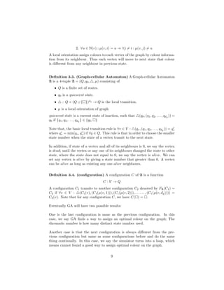
Definition 3.1. Let a graph G = (V, E) be a undirected graph, we use dg for
the degree of G. For every u ∈ V , we denote the set of neighbour by N(v).
The system is based on the colours selected by adjacent vertices of vertices.
The system need to collect neighbours for all vertex.
Definition 3.2. A local orientation is a function µ : V × [1, dg] → (V ∪ { })
where /∈ V and for all v ∈ V . Thus we have rules:
1. N(v) ⊆ {µ(v, i)|i = 1, 2, . . . , dg} ⊆ N(v) ∪ { }
8

9. 2. ∀u ∈ N(v) : µ(v, i) = u ⇒ ∀j = i : µ(v, j) = u
A local orientation assign colours to each vertex of the graph by colour informa-
tion from its neighbour. Thus each vertex will move to next state that colour
is different from any neighbour in pervious state.
Definition 3.3. (Graph-cellular Automaton) A Graph-cellular Automaton
A is a 4-tuple A = (Q, q0, , µ) consisting of
• Q is a finite set of states.
• q0 is a quiescent state.
• : Q × (Q ∪ { })dg
→ Q is the local transition.
• µ is a local orientation of graph
quiescent state is a current state of inaction, such that (q0, (q1, q2, . . . , qdg
)) =
q0 if {q1, q2, . . . , qdg
} ∈ {q0, }
Note that, the basic local transition rule is ∀v ∈ V : (qv, (q1, q2, . . . , qdg )) = qv
where qv = min(qv, qv) if ∀q ∈ Q. This rule is that in order to choose the smaller
state number when the state of a vertex transit to the next state.
In addition, if state of a vertex and all of its neighbours is 0, we say the vertex
is dead; until the vertex or any one of its neighbours changed the state to other
state, where the state does not equal to 0, we say the vertex is alive. We can
set any vertex is alive by giving a state number that greater than 0. A vertex
can be alive as long as existing any one alive neighbours.
Definition 3.4. (configuration) A configuration C of A is a function
C : V → Q
A configuration C1 transits to another configuration C2 denoted by FA(C1) =
C2 if ∀v ∈ V : (C1(v), (C1(µ(v, 1))), (C1(µ(v, 2))), . . . . . . , (C1(µ(v, dg)))) =
C2(v). Note that for any configuration C, we have C( ) = .
Eventually GA will have two possible results:
One is the last configuration is same as the previous configuration. In this
case, we say GA finds a way to assign an optimal colour on the graph; The
chromatic number is how many distinct state number used.
Another case is that the next configuration is always different from the pre-
vious configuration but same as some configurations before and do the same
thing continually. In this case, we say the simulator turns into a loop, which
means cannot found a good way to assign optimal colour on the graph.
9

10. q1
q2
q3
q4
q5
v0
v1 v2
v3
v4v5
v6
v7
(a) in subgraph of G, v0 has 4
neighbours v1, v3, v5 and v7, where
q1 is state of v0, q2 is state of v1,
q3 is state of v3, q4 is state of v5
and q5 is state of v7
q1
q2
q3
q4
q5
v0
v1 v2
v3
v4v5
v6
v7
(b) this figure shows the next con-
figuration represents the state of
v0 transform to q0, and states of
all neighbours of v0 transform to
qi
Figure 5: Example of a configuration
Example 3.5. A graph G = (V, E) is a undirected graph; The degree dg of
G is 7. Figure 5 shows a vertex v0 in a subgraph of G has 4 neighbours. The
vertex has own state q0 ancd for each neighbour has separate state. The next
state of q0 is based on states of N(v). Thus we call FA is global transition.
4 Graph Colouring with GDS
In this section, A Java program is used to simulate colouring with graph dy-
namical system. The program can generate some specified graph, such as linear
graph, circle graph, star graph, wheel graph and peterson graph, or random
graph with giving number of vertex. The simulator will show configurations of
graph.
4.1 implementation of colouring graph with GDS
Colouring graph with GDS simulate on a Java program. The simulator shows a
specified graph with finite vertex. In program a circle represents a vertex, which
use a number to represent the state of a vertex and another number to represent
the index of the vertex. For example, a connected graph with 2 vertices shows
vertex v0 and vertex v1 are both in state 0. Further more, the state number
change to 1 if a vertex is activated. i.e. state of v0 is 1, and its neighbour v1
is 0, which means the transition of v0 is v0
(1, (0)) = 1 and v0
(0, (1)) = 0.
Thus q1 = 1 and q0 = 0 is quiescent state.
10

11. (a) Initialized vertex with state
number under the vertex, and in-
dex number is above the vertex.
(b) state number change to 1 when
vertex of index 0 is activated
Figure 6: Example of the simulator
4.2 Colour some specified case
Case 1: linear graph with odd number of vertex
The simulator initialize a linear graph G with odd number of vertex, like 7 ver-
tices, which the degree of the graph is 2. Every vertex has state number that
indicated as {0, 1, 2, . . . , i} to represent different colour. Each initialized vertex
and its neighbours should be 0, which means all vertices are dead in quiescent
state.
A Graph-cellular Automaton A = (Q, q0, , µ) is running on G, where Q is a
finite set of state, q0 is a quiescent state, is a the local transition and µ is
a local orientation of G. On the initial graph, all vertices is in quiescent state.
However, once any one of vertices is alive and the state of the vertex changed
to other state that does not equal to 0, then the local transition for all vertices
will be affected.
Figure 7 shows each configuration on G. As a neighbour of v1, v0 increase
state to 1, which lead to increasing the state of v1. The configuration to the
next configuration is:
C0 :










(0, ( , 0))
(0, (0, 0)),
(0, (0, 0)),
(0, (0, 0)),
(0, (0, 0)),
(0, (0, 0)),
(0, (0, ))










→ C1 :










(1, ( , 0))
(0, (1, 0)),
(0, (0, 0)),
(0, (0, 0)),
(0, (0, 0)),
(0, (0, 0)),
(0, (0, ))










Thus, v2, v3, . . . , v6 will increase or decrease the state of the vertex by rules
in the following steps. The following configurations is:
11

12. C1 :










(1, ( , 0))
(0, (1, 0)),
(0, (0, 0)),
(0, (0, 0)),
(0, (0, 0)),
(0, (0, 0)),
(0, (0, ))










→ C2 :










(1, ( , 2))
(2, (1, 0)),
(0, (2, 0)),
(0, (0, 0)),
(0, (0, 0)),
(0, (0, 0)),
(0, (0, ))










C2 :










(1, ( , 2))
(2, (1, 0)),
(0, (2, 0)),
(0, (0, 0)),
(0, (0, 0)),
(0, (0, 0)),
(0, (0, ))










→ C3 :










(0, ( , 2))
(2, (0, 1)),
(1, (2, 0)),
(0, (1, 0)),
(0, (0, 0)),
(0, (0, 0)),
(0, (0, ))










C3 :










(0, ( , 2))
(2, (0, 1)),
(1, (2, 0)),
(0, (1, 0)),
(0, (0, 0)),
(0, (0, 0)),
(0, (0, ))










→ C4 :










(0, ( , 2))
(2, (0, 1)),
(1, (2, 2)),
(2, (1, 0)),
(0, (2, 0)),
(0, (0, 0)),
(0, (0, ))










C4 :










(0, ( , 2))
(2, (0, 1)),
(1, (2, 2)),
(2, (1, 0)),
(0, (2, 0)),
(0, (0, 0)),
(0, (0, ))










→ C5 :










(0, ( , 2))
(2, (0, 0)),
(0, (2, 2)),
(2, (0, 1)),
(1, (2, 0)),
(0, (1, 0)),
(0, (0, ))










C5 :










(0, ( , 2))
(2, (0, 0)),
(0, (2, 2)),
(2, (0, 1)),
(1, (2, 0)),
(0, (1, 0)),
(0, (0, ))










→ C6 :










(0, ( , 1))
(1, (0, 0)),
(0, (1, 2)),
(2, (0, 1)),
(1, (2, 2)),
(2, (1, 0)),
(0, (2, ))










C6 :










(0, ( , 1))
(1, (0, 0)),
(0, (1, 2)),
(2, (0, 1)),
(1, (2, 2)),
(2, (1, 0)),
(0, (2, ))










→ C7 :










(0, ( , 1))
(1, (0, 0)),
(0, (1, 2)),
(2, (0, 0)),
(0, (2, 2)),
(2, (0, 0)),
(0, (2, ))










12

13. C7 :










(0, ( , 1))
(1, (0, 0)),
(0, (1, 2)),
(2, (0, 0)),
(0, (2, 2)),
(2, (0, 0)),
(0, (2, ))










→ C8 :










(0, ( , 1))
(1, (0, 0)),
(0, (1, 1)),
(1, (0, 0)),
(0, (1, 1)),
(1, (0, 0)),
(0, (1, ))










C8 :










(0, ( , 1))
(1, (0, 0)),
(0, (1, 1)),
(1, (0, 0)),
(0, (1, 1)),
(1, (0, 0)),
(0, (1, ))










→ C9 :










(0, ( , 1))
(1, (0, 0)),
(0, (1, 1)),
(1, (0, 0)),
(0, (1, 1)),
(1, (0, 0)),
(0, (1, ))










13

14. (a) A graph initialized with 7
vertices. All vertices are dead
and states for all vertices are
{0, 0, 0, 0, 0, 0, 0} in vertex order.
(b) v0 is alive. The state of v0 is
1, then states for all vertices are
{1,0,0,0,0,0,0} in vertex order.
(c) The state of v1 change to 2
in order to be different with its
neighbours.states for all vertices
are {1,2,0,0,0,0,0} in vertex order.
(d) v2 change state to 1 in order to
be different with its neighbours’.
v0 change to a smaller alternative
state number 0. States for all ver-
tices are {0,2,1,0,0,0,0} in vertex
order.
(e) v3 change the state to 2 for
the same reason of v1 in (c). For
all vertex have smallest state num-
ber. States for all vertices are
{0,2,1,2,0,0,0} in vertex order.
(f) v4 change the state to 1 for the
same reason of v2 in (d). v2 change
to a smaller alternative state num-
ber 0. States for all vertices are
{0,2,0,2,1,0,0} in vertex order.
(g) v1 is not in smallest state num-
ber, then decrease to 1. v5 increase
the state number for same reason
as v1 in (c). States for all vertices
are {0,1,0,2,1,2,0} in vertex order.
(h) v4 is not in smallest state num-
ber, then decrease to 0. Thus,all
vertices is in current smallest num-
ber. States for all vertices are
{0,1,0,2,0,2,0} in vertex order.
(i) state for v3 and v5 is not small-
est, then they decrease to 1. States
for all vertices are {0,1,0,1,0,1,0}
in vertex order.
(j) Finally, configuration is same
as previous configuration, which
means all vertices stay in quiescent
state.
Figure 7: Example of a implementation of Graph-cellular Automaton on a linear
graph with odd number of vertex
Finally, the configuration keep the same as previous configuration, we say
colouring is completed. Because the linear graph with odd number of vertex is
symmetrical with the middle vertex, to start with the first vertex or the last
vertex will have same result. The chromic number is 2
Case 2: linear graph with even number of vertex
In this case, the simulator initialize a linear graph G with even number of vertex,
like 8 vertices, which the degree of the graph is 2. For all initialized vertices and
14

15. neighbours also are 0, which means all vertices are dead in quiescent state.
Figure 8 shows each configuration on G. We try a higher start state number
on v0 to see the final result. The configuration of G with start state number 5
on v0 is:
C0 :












(0, ( , 0))
(0, (0, 0)),
(0, (0, 0)),
(0, (0, 0)),
(0, (0, 0)),
(0, (0, 0)),
(0, (0, 0)),
(0, (0, ))












→ C1 :












(5, ( , 0))
(0, (5, 0)),
(0, (0, 0)),
(0, (0, 0)),
(0, (0, 0)),
(0, (0, 0)),
(0, (0, 0)),
(0, (0, ))












From configuration C1 we have neighbours of v1 has alive vertex, then v1 will
increase state number by local transition. Then we have configuration C2. Even-
tually, we have each configuration as following steps:
C1 :












(5, ( , 0))
(0, (5, 0)),
(0, (0, 0)),
(0, (0, 0)),
(0, (0, 0)),
(0, (0, 0)),
(0, (0, 0)),
(0, (0, ))












→ C2 :












(4, ( , 1))
(1, (4, 0)),
(0, (1, 0)),
(0, (0, 0)),
(0, (0, 0)),
(0, (0, 0)),
(0, (0, 0)),
(0, (0, ))












C2 :












(4, ( , 1))
(1, (4, 0)),
(0, (1, 0)),
(0, (0, 0)),
(0, (0, 0)),
(0, (0, 0)),
(0, (0, 0)),
(0, (0, ))












→ C3 :












(3, ( , 2))
(1, (3, 2)),
(2, (1, 0)),
(0, (2, 0)),
(0, (0, 0)),
(0, (0, 0)),
(0, (0, 0)),
(0, (0, ))












C3 :












(2, ( , 2))
(1, (3, 2)),
(2, (1, 0)),
(0, (2, 0)),
(0, (0, 0)),
(0, (0, 0)),
(0, (0, 0)),
(0, (0, ))












→ C4 :












(2, ( , 0))
(0, (2, 2)),
(2, (0, 1)),
(1, (2, 0)),
(0, (1, 0)),
(0, (0, 0)),
(0, (0, 0)),
(0, (0, ))












15

16. C4 :












(2, ( , 0))
(0, (2, 2)),
(2, (0, 1)),
(1, (2, 0)),
(0, (1, 0)),
(0, (0, 0)),
(0, (0, 0)),
(0, (0, ))












→ C5 :












(1, ( , 0))
(0, (1, 2)),
(2, (0, 1)),
(1, (2, 2)),
(2, (1, 0)),
(0, (2, 0)),
(0, (0, 0)),
(0, (0, ))












C5 :














(1, ( , 0))
(0, (1, 2)),
(2, (0, 1)),
(1, (2, 2)),
(2, (1, 0)),
(0, (2, 0)),
(0, (0, 0)),
(0, (0, 0)),
(0, (0, ))














→ C6 :












(1, ( , 0))
(0, (1, 2)),
(2, (0, 0)),
(0, (2, 2)),
(2, (0, 1)),
(1, (2, 0)),
(0, (0, 0)),
(0, (0, ))












C6 :












(1, ( , 0))
(0, (1, 2)),
(2, (0, 0)),
(0, (2, 2)),
(2, (0, 1)),
(1, (2, 0)),
(0, (0, 0)),
(0, (0, ))












→ C7 :












(1, ( , 0))
(0, (1, 1)),
(1, (0, 0)),
(0, (1, 2)),
(2, (0, 1)),
(1, (2, 2)),
(2, (1, 0)),
(0, (2, ))












C7 :












(1, ( , 0))
(0, (1, 1)),
(1, (0, 0)),
(0, (1, 2)),
(2, (0, 1)),
(1, (2, 2)),
(2, (1, 0)),
(0, (2, ))












→ C8 :












(1, ( , 0))
(0, (1, 1)),
(1, (0, 0)),
(0, (1, 2)),
(2, (0, 0)),
(0, (2, 2)),
(2, (0, 0)),
(0, (2, ))












C8 :












(1, ( , 1))
(0, (1, 1)),
(1, (0, 0)),
(0, (1, 2)),
(2, (0, 0)),
(0, (2, 2)),
(2, (0, 0)),
(0, (2, ))












→ C9 :












(1, ( , 0))
(0, (1, 1)),
(1, (0, 0)),
(0, (1, 1)),
(1, (0, 0)),
(0, (1, 1)),
(1, (0, 0)),
(0, (1, ))












16

17. C9 :












(1, ( , 0))
(0, (1, 1)),
(1, (0, 0)),
(0, (1, 1)),
(1, (0, 0)),
(0, (1, 1)),
(1, (0, 0)),
(0, (1, ))












→ C10 :












(1, ( , 0))
(0, (1, 1)),
(1, (0, 0)),
(0, (1, 1)),
(1, (0, 0)),
(0, (1, 1)),
(1, (0, 0)),
(0, (1, ))












17

18. (a) A graph initialized with 8 ver-
tices. For all vertices are dead.
Thus states for all vertices are
{0, 0, 0, 0, 0, 0, 0, 0} in vertex order.
(b) Increasing state number of
v0 to 5 for colouring yellow.
then states for all vertices are
{5,0,0,0,0,0,0,0} in vertex order.
(c) The state of v0 has possible
smaller state number, 5−1 = 4, for
colouring blue. v1 has alive neigh-
bour, then increase state number
to 1. States for all vertices are
{4,1,0,0,0,0,0,0} in vertex order.
(d) v0 still has possible state num-
ber, 4 − 1 = 3, for colouring green.
alive v1 make v2 increasing state
number to 2. States for all ver-
tices are {3,1,2,0,0,0,0,0} in vertex
order.
(e) v0 decrease state number to
2 for colouring red. From neigh-
bours of v1 knows v1 has possi-
ble smaller number 0. States for
all vertices are {2,0,2,1,0,0,0,0} in
vertex order.
(f) v0 decrease state number to
1. From neighbours of v4 knows
v4 can be alive and increase state
number to 2. States for all ver-
tices are {1,0,2,1,2,0,0,0} in vertex
order.
(g) Neighbours of v3 both are in
state number 2, so v3 change the
state number to smaller possible
number. v5 has alive neighbour,
also can increase state number
to 1. States for all vertices are
{1,0,2,0,2,1,0,0} in vertex order.
(h) v2 is not in smallest state num-
ber, then decrease to 1. v6 also can
be alive and change the state num-
ber to 2. States for all vertices are
{1,0,1,0,2,1,2,0} in vertex order.
(i) state for v5 has two alive neigh-
bour and both in 2. v5 choose a
smaller state number 0. States for
all vertices are {1,0,1,0,2,0,2,0} in
vertex order.
(j) v4 and v6 both have smaller
state number, then turn it into
1.States for all vertices are
{1,0,1,0,1,0,1,0} in vertex order.
(k) Finally, configuration is same
as previous configuration, which
means all vertices stay in quiescent
state.
Figure 8: Example of a implementation of Graph-cellular Automaton on a linear
graph with even number of vertex
18

19. Finally, the configuration keep the same as previous configuration, we say
colouring is completed. The simulator find a good way to assign a optimal
colour on the graph. At the last configuration, we know 2 state numbers is
used. Therefore, the chromatic number is 2.
Case 3: circle graph with even number of vertex
In this case, circle graph with even number of vertex has symmetrical path to
touch the vertex that the index is half of size, such as 2 in 4 vertices, 4 in 8
vertices. The symmetrical vertex on each path can merge into a linear graph
with odd number of vertex. Thus, colouring can be same as linear graph with
odd number of vertex.
Figure 9 shows each configuration on G. Both side of path have symmetri-
cal vertices which turn into same state number. Start with any one of vertices
to end with the opposite vertex through both side of path at the same time.
Following configuration shown as steps:
C0 :












(0, (0, 0))
(0, (0, 0)),
(0, (0, 0)),
(0, (0, 0)),
(0, (0, 0)),
(0, (0, 0)),
(0, (0, 0)),
(0, (0, 0))












→ C1 :












(1, (0, 0))
(0, (1, 0)),
(0, (1, 0)),
(0, (0, 0)),
(0, (0, 0)),
(0, (0, 0)),
(0, (0, 0)),
(0, (0, 1))












C1 :












(1, (0, 0))
(0, (1, 0)),
(0, (0, 0)),
(0, (0, 0)),
(0, (0, 0)),
(0, (0, 0)),
(0, (0, 0)),
(0, (0, 1))












→ C2 :












(1, (2, 2))
(2, (1, 0)),
(0, (2, 0)),
(0, (0, 0)),
(0, (0, 0)),
(0, (0, 0)),
(0, (0, 2)),
(2, (0, 1))












C2 :












(1, (2, 2))
(2, (1, 0)),
(0, (2, 0)),
(0, (0, 0)),
(0, (0, 0)),
(0, (0, 0)),
(0, (0, 2)),
(2, (0, 1))












→ C3 :












(0, (2, 2))
(2, (0, 1)),
(1, (2, 0)),
(0, (1, 0)),
(0, (0, 0)),
(0, (0, 1)),
(1, (0, 2)),
(2, (1, 0))












19

20. C3 :












(0, (2, 2))
(2, (0, 1)),
(1, (2, 0)),
(0, (1, 0)),
(0, (0, 0)),
(0, (0, 1)),
(1, (0, 2)),
(2, (1, 0))












→ C4 :












(0, (2, 2))
(2, (0, 1)),
(1, (2, 2)),
(0, (1, 0)),
(0, (0, 0)),
(0, (0, 1)),
(1, (2, 2)),
(2, (1, 0))












C4 :












(0, (2, 2))
(2, (0, 1)),
(1, (2, 2)),
(0, (1, 0)),
(0, (0, 0)),
(0, (0, 1)),
(1, (2, 2)),
(2, (1, 0))












→ C5 :












(0, (2, 2))
(2, (0, 1)),
(1, (2, 2)),
(2, (1, 0)),
(0, (2, 2)),
(2, (0, 1)),
(1, (2, 2)),
(2, (1, 0))












C5 :












(0, (2, 2))
(2, (0, 1)),
(1, (2, 2)),
(2, (1, 0)),
(0, (2, 2)),
(2, (0, 1)),
(1, (2, 2)),
(2, (1, 0))












→ C6 :












(0, (2, 2))
(2, (0, 0)),
(0, (2, 2)),
(2, (0, 0)),
(0, (2, 2)),
(2, (0, 0)),
(0, (2, 2)),
(2, (0, 0))












C6 :












(0, (2, 2))
(2, (0, 0)),
(0, (2, 2)),
(2, (0, 0)),
(0, (2, 2)),
(2, (0, 0)),
(0, (2, 2)),
(2, (0, 0))












→ C7 :












(0, (1, 1))
(1, (0, 0)),
(0, (1, 1)),
(1, (0, 0)),
(0, (1, 1)),
(1, (0, 0)),
(0, (1, 1)),
(1, (0, 0))












C7 :












(0, (1, 1))
(1, (0, 0)),
(0, (1, 1)),
(1, (0, 0)),
(0, (1, 1)),
(1, (0, 0)),
(0, (1, 1)),
(1, (0, 0))












→ C8 :












(0, (1, 1))
(1, (0, 0)),
(0, (1, 1)),
(1, (0, 0)),
(0, (1, 1)),
(1, (0, 0)),
(0, (1, 1)),
(1, (0, 0))












Finally, the configuration keep the same as previous configuration, we say colour-
ing is completed. Any linear graph with even number of vertex, n > 2, the
20

21. system will have same result through same local transition. The simulator find
a good way to assign a optimal colour on the graph. At the last configuration,
we know 2 state numbers is used. Therefore, the chromatic number is 2.
21

22. (a) A graph initialized
with 8 vertices. For all
vertices are dead. Thus
state for all vertices are
{0,0,0,0,0,0,0,0} in index
of vertex order.
(b) Increase state number
of v0 to 1 for mak-
ing the vertex alive.
State for all vertices are
{1,0,0,0,0,0,0,0} in index
of vertex order.
(c) Symmetrical vertices
v1 and v7 both has alive
vertex v0, then they both
increase state number to
2. State for all vertices
are {1,2,0,0,0,0,0,2} in in-
dex of vertex order.
(d) Both side of v0 has
state number 2, so 0 be-
come to a possible smaller
number for v0. Symmet-
rical vertices v2 and v6
change state number to 1.
State for all vertices are
{0,2,1,0,0,0,1,2}
(e) Symmetrical ver-
tices v3 and v5 increase
state number to 2.
State for all vertices are
{0,2,1,2,0,2,1,2} in index
of vertex order.
(f) neighbours of both
side for symmetrical ver-
tices v2 and v6 have state
number 2, thus 0 become
to possible smaller num-
ber. State for all vertices
are {0,2,0,2,0,2,0,2} in in-
dex of vertex order.
(g) All neighbours of
v1, v3, v5, v7 has state
number 0, Thus they
decrease state numbers
to 1. State for all vertices
are {0,1,0,1,0,1,0,1} in
index of vertex order.
(h) Finally, configuration
is same as previous config-
uration, which means all
vertices stay in quiescent
state.
Figure 9: Example of a implementation of Graph-cellular Automaton on a circle
graph with even number of vertex
22

23. Case 4: circle graph with odd number of vertex
In this case, we need to consider the smallest circle graph with odd number of
vertex, which the graph with 3 vertices. Because any larger circle graph with
odd number of vertex is start from the endpoint to the other two endpoints
through two symmetrical path. If the simulator can run on the smallest graph
well, then it also can run any larger circle graph with odd number of vertex. The
graph G is a triangle. Start with any one of vertices, other two vertices must
has same local transition. However the two vertices are also connected together.
So, in this situation, the two vertices cannot have a good proper colouring. The
simulator will turn into a dynamic balance.
C0 :


(0, (0, 0))
(0, (0, 0)),
(0, (0, 0))

 → C1 :


(1, (0, 0))
(0, (1, 0)),
(0, (1, 0))


C1 :


(1, (0, 0))
(0, (1, 0)),
(0, (1, 0))

 → C2 :


(1, (2, 2))
(2, (1, 2)),
(2, (1, 2))


C2 :


(1, (2, 2))
(2, (1, 2)),
(2, (1, 2))

 → C3 :


(0, (2, 2))
(2, (0, 2)),
(2, (0, 2))


C3 :


(0, (2, 2))
(2, (0, 2)),
(2, (0, 2))

 → C4 :


(0, (1, 1))
(1, (0, 1)),
(1, (0, 1))


C3 :


(0, (1, 1))
(1, (0, 1)),
(1, (0, 1))

 → C4 :


(0, (2, 2))
(2, (0, 2)),
(2, (0, 2))


...
...
Configuration as above shows the simulator turn into a infinite loop. The sim-
ulator cannot find a good way to assign proper colour for all vertices on the
graph. Figure 10 shows a example how turn into a dynamic balance. In step
10(f) repeatedly do what step 10(d) did. Thus the simulator is in a loop.
23

24. (a) A graph initialized circle graph
with 3 vertices. For all vertices are
dead. Thus state for all vertices
are {0,0,0} in index of vertex or-
der.
(b) We start with any vertex, e.g.
v0. State for all vertices are
{1,0,0} in index of vertex order.
(c) v0 is neighbour of v1 and v2,
and v1, v2 is adjacent. v1, v2 both
have neighbours that in state num-
ber 1 and 0. So they increase state
number to 2 together at the same
time. State for all vertices are
{1,2,2} in index of vertex order.
(d) All neighbours of v0 is in state
2. v0 choose the smallest state
number 0. State for all vertices are
{0,2,2} in index of vertex order.
(e) v1, v2 have a smaller choice,
state 1. State for all vertices are
{0,2,2} in index of vertex order.
(f) v1, v2 increase their state num-
ber for the same reason in (d).
State for all vertices are {0,2,2} in
index of vertex order. The simula-
tor turn into a infinite loop.
Figure 10: Example of a implementation of Graph-cellular Automaton on a
circle graph
24

25. Case 5: star graph
In this case, star graph is a graph made up of a single vertex v in the middle
and all the other vertices hanging off it; these vertices are connected only to the
centre. For the reason, if start vertex is the centre vertex, then the graph will
have a good proper colouring, Otherwise after some configuration also have a
good proper colouring.
Figure 11 shows each configuration on the star graph G. Start with the centre
vertex or any components of the connected neighbours, the star graph G will
has a good proper colouring. The configurations is following:
C0 :












(0, (0, 0, 0, 0, 0))
(0, (0, , , , , )),
(0, (0, , , , , )),
(0, (0, , , , , )),
(0, (0, , , , , )),
(0, (0, , , , , )),
(0, (0, , , , , )),
(0, (0, , , , , ))












→ C1 :












(0, (0, 0, 0, 0, 0))
(1, (0, , , , , )),
(0, (0, , , , , )),
(0, (0, , , , , )),
(0, (0, , , , , )),
(0, (0, , , , , )),
(0, (0, , , , , )),
(0, (0, , , , , ))












C1 :












(0, (0, 0, 0, 0, 0))
(1, (0, , , , , )),
(0, (0, , , , , )),
(0, (0, , , , , )),
(0, (0, , , , , )),
(0, (0, , , , , )),
(0, (0, , , , , )),
(0, (0, , , , , ))












→ C2 :












(2, (1, 0, 0, 0, 0))
(1, (2, , , , , )),
(0, (0, , , , , )),
(0, (0, , , , , )),
(0, (0, , , , , )),
(0, (0, , , , , )),
(0, (0, , , , , )),
(0, (0, , , , , ))












C2 :












(2, (1, 0, 0, 0, 0))
(1, (2, , , , , )),
(0, (0, , , , , )),
(0, (0, , , , , )),
(0, (0, , , , , )),
(0, (0, , , , , )),
(0, (0, , , , , )),
(0, (0, , , , , ))












→ C3 :












(2, (0, 0, 0, 0, 0))
(0, (2, , , , , )),
(0, (0, , , , , )),
(0, (0, , , , , )),
(0, (0, , , , , )),
(0, (0, , , , , )),
(0, (0, , , , , )),
(0, (0, , , , , ))












C3 :












(2, (0, 0, 0, 0, 0))
(0, (2, , , , , )),
(0, (0, , , , , )),
(0, (0, , , , , )),
(0, (0, , , , , )),
(0, (0, , , , , )),
(0, (0, , , , , )),
(0, (0, , , , , ))












→ C4 :












(1, (0, 0, 0, 0, 0))
(0, (1, , , , , )),
(0, (0, , , , , )),
(0, (0, , , , , )),
(0, (0, , , , , )),
(0, (0, , , , , )),
(0, (0, , , , , )),
(0, (0, , , , , ))












25

26. C4 :












(1, (0, 0, 0, 0, 0))
(0, (1, , , , , )),
(0, (0, , , , , )),
(0, (0, , , , , )),
(0, (0, , , , , )),
(0, (0, , , , , )),
(0, (0, , , , , )),
(0, (0, , , , , ))












→ C5 :












(1, (0, 0, 0, 0, 0))
(0, (1, , , , , )),
(0, (0, , , , , )),
(0, (0, , , , , )),
(0, (0, , , , , )),
(0, (0, , , , , )),
(0, (0, , , , , )),
(0, (0, , , , , ))












26

27. (a) A graph initialized
with 6 vertices. For all
vertices are dead. Thus
state for all vertices are
{0,0,0,0,0,0} in index of
vertex order.
(b) Increase state number
of v1 to 1 for making the
vertex alive. State for all
vertices are {0,1,0,0,0,0}
in index of vertex order.
(c) The center vertex con-
nected to the alive ver-
tex, then the center ver-
tex increase state number
to 2. State for all vertices
are {2,1,0,0,0,0} in index
of vertex order.
(d) To compare with the
center vertex, the start
state has possible smaller
state number. So the ver-
tex decrease state number
to 0. State for all vertices
are {2,0,0,0,0,0}
(e) All neighbours of the
center vertex is in 0
state number. The cen-
ter vertex decrease the
state number to the pos-
sible smallest numebr 1.
State for all vertices are
{1,0,0,0,0,0} in index of
vertex order.
(f) Finally, configuration
is same as previous config-
uration, which means all
vertices stay in quiescent
state.
Figure 11: Example of a implementation of Graph-cellular Automaton on a star
graph
Finally, the configuration keep the same as previous configuration, we say
colouring is completed. Because any one of components neighbours are equiv-
27

28. alent. Then to start with any one of them will have same result. The Graph-
cellular automaton obtain proposed colour via starting with the any one or more
vertices. The chromic number is 2.
Case 6: wheel graph
In this case, wheel graph contains circle graph with odd number of vertex. We
already know if any graph contains odd number of vertex, the graph will turn
into a dynamic balance.
Figure 12 shows the graph-cellular automaton turn into a dynamic balance.
The simulator repeatedly turn into a loop between (d) and (e) forever. The
configuration is following:
C0 :




(0, (0, 0, 0))
(0, (0, 0, 0)),
(0, (0, 0, 0)),
(0, (0, 0, 0)))



 → C1 :




(0, (1, 0, 0))
(1, (0, 0, 0)),
(0, (0, 1, 0)),
(0, (0, 1, 0)))




C1 :




(0, (1, 0, 0))
(1, (0, 0, 0)),
(0, (0, 1, 0)),
(0, (0, 1, 0)))



 → C2 :




(2, (1, 2, 2))
(1, (2, 2, 2)),
(2, (2, 1, 2)),
(2, (2, 1, 2)))




C2 :




(2, (1, 2, 2))
(1, (2, 2, 2)),
(2, (2, 1, 2)),
(2, (2, 1, 2)))



 → C3 :




(2, (0, 2, 2))
(0, (2, 2, 2)),
(2, (2, 0, 2)),
(2, (2, 0, 2)))




C3 :




(2, (0, 2, 2))
(0, (2, 2, 2)),
(2, (2, 0, 2)),
(2, (2, 0, 2)))



 → C4 :




(1, (0, 1, 1))
(0, (1, 1, 1)),
(1, (1, 0, 1)),
(1, (1, 0, 1)))




C4 :




(1, (0, 1, 1))
(0, (1, 1, 1)),
(1, (1, 0, 1)),
(1, (1, 0, 1)))



 → C3 :




(2, (0, 2, 2))
(0, (2, 2, 2)),
(2, (2, 0, 2)),
(2, (2, 0, 2)))




...
...
28

29. (a) A graph initialized with 4 ver-
tices. For all vertices are dead.
Thus state for all vertices are
{0,0,0,0} in index of vertex order.
(b) Increase state number of v1
to 1 for making the vertex alive.
State for all vertices are {0,1,0,0,}
in index of vertex order.
(c) The start vertex v1 connected
to 3 vertices, then neighbours in-
crease the state number to 2. State
for all vertices are {2,1,2,2} in in-
dex of vertex order.
(d) All neighbour of v1 increased
state number to 2, the vertex de-
crease to possible smaller num-
ber 0. State for all vertices are
{2,0,2,2}
(e) Neighbours of v1 connected
each other. Thus they choose a
possible smaller state number to 1
together at the same time. State
for all vertices are {1,0,1,1} in in-
dex of vertex order.
(f) Neighbours of v1 have to select
different colour from each other.
But the neighbours of them select
0 and 1, thus they increase state
number to 2 together at the same
time. This step is repeat of previ-
ous step.
Figure 12: Example of a implementation of Graph-cellular Automaton on a
wheel graph
Finally, the Graph-cellular automaton cannot find a proper colouring for
wheel graph. Because the graph-cellular automaton is imperfectness on circle
graph and wheel graph usually exists circle graph with odd number of vertex.
29

30. Case 7: Peterson graph
In this section, peterson graph is a special and more complicated graph. It is
hard to find a solution from only one start vertex. Therefore, to start with
colouring graph, we usually pick a independent set of the graph. For each
neighbours of the vertices in independent set choose a optimal colour based on
the adjacent vertex.
C0 :
















(0, (0, , , 0, 0, , , , ))
(0, (0, 0, , , , 0, , , )),
(0, ( , 0, 0, , , , 0, , )),
(0, ( , , 0, 0, , , , 0, )))
(0, (0, , , 0, , , , , 0)))
(0, (0, , , , , , 0, 0, )))
(0, ( , 0, , , , , , 0, 0)))
(0, ( , , 0, , , 0, , , 0)))
(0, ( , , , 0, , 0, 0, , )))
(0, ( , , , , 0, , 0, 0, )))
















→ C1 :
















(1, (0, , , 0, 0, , , , ))
(0, (1, 0, , , , 1, , , )),
(0, ( , 0, 1, , , , 1, , )),
(1, ( , , 0, 0, , , , 0, )))
(0, (1, , , 1, , , , , 0)))
(0, (1, , , , , , 1, 0, )))
(1, ( , 0, , , , , , 0, 0)))
(1, ( , , 0, , , 0, , , 0)))
(0, ( , , , 1, , 0, 1, , )))
(0, ( , , , , 0, , 1, 1, )))
















C1 :
















(1, (0, , , 0, 0, , , , ))
(0, (1, 0, , , , 1, , , )),
(0, ( , 0, 1, , , , 1, , )),
(1, ( , , 0, 0, , , , 0, )))
(0, (1, , , 1, , , , , 0)))
(0, (1, , , , , , 1, 0, )))
(1, ( , 0, , , , , , 0, 0)))
(1, ( , , 0, , , 0, , , 0)))
(0, ( , , , 1, , 0, 1, , )))
(0, ( , , , , 0, , 1, 1, )))
















→ C2 :
















(1, (2, , , 2, 2, , , , ))
(2, (1, 2, , , , 1, , , )),
(2, ( , 2, 1, , , , 1, , )),
(1, ( , , 2, 2, , , , 2, )))
(2, (1, , , 1, , , , , 2)))
(2, (1, , , , , , 1, 2, )))
(1, ( , 2, , , , , , 2, 2)))
(1, ( , , 2, , , 2, , , 2)))
(2, ( , , , 1, , 2, 1, , )))
(2, ( , , , , 2, , 1, 1, )))
















C2 :
















(1, (2, , , 2, 2, , , , ))
(2, (1, 2, , , , 1, , , )),
(2, ( , 2, 1, , , , 1, , )),
(1, ( , , 2, 2, , , , 2, )))
(2, (1, , , 1, , , , , 2)))
(2, (1, , , , , , 1, 2, )))
(1, ( , 2, , , , , , 2, 2)))
(1, ( , , 2, , , 2, , , 2)))
(2, ( , , , 1, , 2, 1, , )))
(2, ( , , , , 2, , 1, 1, )))
















→ C3 :
















(0, (2, , , 2, 2, , , , ))
(2, (0, 2, , , , 0, , , )),
(2, ( , 2, 0, , , , 0, , )),
(0, ( , , 2, 2, , , , 2, )))
(2, (0, , , 0, , , , , 2)))
(2, (0, , , , , , 0, 2, )))
(0, ( , 2, , , , , , 2, 2)))
(0, ( , , 2, , , 2, , , 2)))
(2, ( , , , 0, , 2, 0, , )))
(2, ( , , , , 2, , 0, 0, )))
















C3 :
















(0, (2, , , 2, 2, , , , ))
(2, (0, 2, , , , 0, , , )),
(2, ( , 2, 0, , , , 0, , )),
(0, ( , , 2, 2, , , , 2, )))
(2, (0, , , 0, , , , , 2)))
(2, (0, , , , , , 0, 2, )))
(0, ( , 2, , , , , , 2, 2)))
(0, ( , , 2, , , 2, , , 2)))
(2, ( , , , 0, , 2, 0, , )))
(2, ( , , , , 2, , 0, 0, )))
















→ C4 :
















(0, (1, , , 1, 1, , , , ))
(1, (0, 1, , , , 0, , , )),
(1, ( , 1, 0, , , , 0, , )),
(0, ( , , 1, 1, , , , 1, )))
(1, (0, , , 0, , , , , 1)))
(1, (0, , , , , , 0, 1, )))
(0, ( , 1, , , , , , 1, 1)))
(0, ( , , 1, , , 1, , , 1)))
(1, ( , , , 0, , 1, 0, , )))
(1, ( , , , , 1, , 0, 0, )))
















30

31. C4 :
















(0, (1, , , 1, 1, , , , ))
(1, (0, 1, , , , 0, , , )),
(1, ( , 1, 0, , , , 0, , )),
(0, ( , , 1, 1, , , , 1, )))
(1, (0, , , 0, , , , , 1)))
(1, (0, , , , , , 0, 1, )))
(0, ( , 1, , , , , , 1, 1)))
(0, ( , , 1, , , 1, , , 1)))
(1, ( , , , 0, , 1, 0, , )))
(1, ( , , , , 1, , 0, 0, )))
















→ C3 :
















(0, (2, , , 2, 2, , , , ))
(2, (0, 2, , , , 0, , , )),
(2, ( , 2, 0, , , , 0, , )),
(0, ( , , 2, 2, , , , 2, )))
(2, (0, , , 0, , , , , 2)))
(2, (0, , , , , , 0, 2, )))
(0, ( , 2, , , , , , 2, 2)))
(0, ( , , 2, , , 2, , , 2)))
(2, ( , , , 0, , 2, 0, , )))
(2, ( , , , , 2, , 0, 0, )))
















...
...
31

32. (a) A graph initialized peterson
graph with 10 vertices. For all ver-
tices are dead. Thus state for all
vertices are {0,0,0,0,0,0,0,0,0,0} in
index of vertex order.
(b) Making some vertice alive in a
independent set of G. State for all
vertices are {1,0,0,1,0,0,1,1,0,0} in
index of vertex order.
(c) All neighbours of chosen ver-
tices are increase the state num-
ber to 2. State for all vertices
are {1,2,2,1,2,2,1,1,2,2} in index of
vertex order.
(d) In previous step, vertices
choose a optimal colouring by
their adjacent vertices, then they
change state number together at
the same time. State for all ver-
tices are {0,2,2,0,2,2,0,0,2,2} in in-
dex of vertex order.
(e) The neighbours of independent
set decrease state number to 1 to-
gether at the same time. State for
all vertices are {0,1,1,0,1,1,0,0,1,1}
in index of vertex order.
(f) The neighbours of indepen-
dent set choose by their adjacent
vertices. They all have neigh-
bours in 0 and 1, so they in-
crease to 2. State for all vertices
are {0,2,2,0,2,2,0,0,2,2} in index of
vertex order.
Figure 13: Example of a implementation of Graph-cellular Automaton on a
peterson graph
32

33. Finally, the Graph-cellular automaton cannot find a proper colouring for
peterson graph. The graph-cellular automaton cannot cover all classed of graph.
Thus the problem new is to extend this model to more general classes of graphs.
We would like to develop this and try obtain some more reliable result.
5 Conclusion
In this report, a graph-cellular automaton was proposed for finding a possible
optimal solution to the vertex colouring problem. Graph-cellular automaton is
a model of graph dynamical system, which is a distributed system that each
vertex choose its optimal colour based on the colours selected by its adjacent
vertices. We use a simulation to find a way to colour linear graph and circle
graph with even number of vertex that is more than 2 vertices. The result for
each specific case is:
• Linear graph
– Linear graph with odd number of vertex: The Graph-cellular
automaton successfully found a proper colouring for any linear graph
with odd number of vertex via starting with any one or more vertices.
– Linear graph with even number of vertex: The Graph-cellular
automaton successfully found a proper colouring for any linear graph
with even number of vertex via starting with any one or more vertices.
• Circle graph
– Circle graph with odd number of vertex: The Graph-cellular
automaton cannot find a proper colouring for circle graph with odd
number of vertex.
– Circle graph with even number of vertex: The Graph-cellular
automaton successfully found a proper colouring for any linear graph
with even number of vertex via starting with any one or more vertices.
• Star graph: The Graph-cellular automaton successfully found a proper
colouring for any star graph via starting with any one or more vertices.
• Wheel graph: Due to imperfectness on circle, the Graph-cellular au-
tomaton cannot find a proper colouring for wheel graph existing circle
graph with odd number of vertex.
33

34. • Peterson graph: The Graph-cellular automaton cannot find a proper
colouring for peterson graph.
The obtained results showed that the simple graph-cellular automaton is not
appropriate for colouring circle graph with 3 vertices well, which means only a
simple graph-cellular automaton model might not solve all graph.
Our aim is to investigate the possibility of solving the vertex colouring problem
on graph using cellular automata. The case studies show that graph dynamical
system can be used as a viable tool in obtaining a colouring for specific classes
of graph. The natural problem now is to extend this work to more general
classes of graphs. As a next step, we would like to investigate this more general
problem and try obtain some more generic faces.
34

35. References
[1] Javad Akbari Torkestani and Mohammad Reza Meybodi. A cellular learn-
ing automata-based algorithm for solving the vertex coloring problem. Ex-
pert Systems with Applications, 38(8):9237–9247, 2011.
[2] Nicolas Barnier and Pascal Brisset. Graph coloring for air traffic flow man-
agement. Annals of operations research, 130(1-4):163–178, 2004.
[3] Kenneth P Bogart. Introductory combinatorics. Saunders College Publish-
ing, 1989.
[4] Preston Briggs. Register allocation via graph coloring. PhD thesis, Rice
University, 1992.
[5] Reinhard Diestel. Graph theory. 2005, 2005.
[6] Marek Kubale. Graph colorings, volume 352. American Mathematical Soc.,
2004.
[7] Bruce Montgomery. Dynamic coloring of graphs. PhD thesis, West Virginia
University, 2001.
[8] Palash Sarkar. A brief history of cellular automata. ACM Comput. Surv.,
32(1):80–107, March 2000.
[9] Michael Sipser. Introduction to the Theory of Computation, volume 2.
Thomson Course Technology Boston, 2006.
[10] Stephen Wolfram. Cellular automata and complexity: collected papers, vol-
ume 1. Addison-Wesley Reading, 1994.
35