This document discusses linear programming formulations for inventory management decision problems with service constraints under uncertainty. It addresses situations where the probability distribution of demand during lead times is incompletely known. The document defines two key performance measures - expected shortage per replenishment cycle and probability of stock-out during lead time. It states that when distribution information is incomplete, these measures can only be bounded rather than determined with a single value. The document proposes formulating an optimization model to determine a safety stock level that guarantees meeting the performance measures under the worst case lead time demand scenario.

1. Linear programming formulation in inventory
management decision problems with a service
constraint
By: Asaye Dessie
Linear programming formulation in inventory
management decision problems with a service
constraint
By: Asaye Dessie

2. A B S T R A C T
 Inventory systems with uncertainty go hand in hand with the
determination of a safety stock level.
 The decision on the safety stock level is based on a performance measure,
for example the expected shortage per replenishment period or the
probability of a stock-out per replenishment period.
 The performance measure assumes complete knowledge of the
probability distribution during lead time, which might not be available.
 In case of incomplete information regarding the lead-time distribution of
demand, no single figure for the safety stock can be determined in order
to satisfy a performance measure.
 However, an optimization model may be formulated in order to determine
a safety stock level which guarantees the performance measure under the
worst case of lead-time demand, of which the distribution is known in an
incomplete way.
 It is shown that this optimization problem can be formulated as a linear
programming problem.
 Inventory systems with uncertainty go hand in hand with the
determination of a safety stock level.
 The decision on the safety stock level is based on a performance measure,
for example the expected shortage per replenishment period or the
probability of a stock-out per replenishment period.
 The performance measure assumes complete knowledge of the
probability distribution during lead time, which might not be available.
 In case of incomplete information regarding the lead-time distribution of
demand, no single figure for the safety stock can be determined in order
to satisfy a performance measure.
 However, an optimization model may be formulated in order to determine
a safety stock level which guarantees the performance measure under the
worst case of lead-time demand, of which the distribution is known in an
incomplete way.
 It is shown that this optimization problem can be formulated as a linear
programming problem.

3. 1. Introduction
Some uncertainty in an inventory system (such as lead time, quantity and
quality) depends on the suppliers.
If the suppliers introduce too much uncertainty, corrective action should be
taken.
Some uncertainty, however, is attributable to customers, especially
demand.
If insufficient inventory is hold, a stock-out may occur leading to shortage
costs.
Shortage costs are usually high in relation to holding costs.
Companies are willing to hold additional inventory, above their forecasted
needs, to add a margin of safety.
Some uncertainty in an inventory system (such as lead time, quantity and
quality) depends on the suppliers.
If the suppliers introduce too much uncertainty, corrective action should be
taken.
Some uncertainty, however, is attributable to customers, especially
demand.
If insufficient inventory is hold, a stock-out may occur leading to shortage
costs.
Shortage costs are usually high in relation to holding costs.
Companies are willing to hold additional inventory, above their forecasted
needs, to add a margin of safety.
Some uncertainty in an inventory system (such as lead time, quantity and
quality) depends on the suppliers.
If the suppliers introduce too much uncertainty, corrective action should be
taken.
Some uncertainty, however, is attributable to customers, especially
demand.
If insufficient inventory is hold, a stock-out may occur leading to shortage
costs.
Shortage costs are usually high in relation to holding costs.
Companies are willing to hold additional inventory, above their forecasted
needs, to add a margin of safety.
Some uncertainty in an inventory system (such as lead time, quantity and
quality) depends on the suppliers.
If the suppliers introduce too much uncertainty, corrective action should be
taken.
Some uncertainty, however, is attributable to customers, especially
demand.
If insufficient inventory is hold, a stock-out may occur leading to shortage
costs.
Shortage costs are usually high in relation to holding costs.
Companies are willing to hold additional inventory, above their forecasted
needs, to add a margin of safety.

4. Cont…
Determination of an inventory replenishment policy, of the quantities to order,
of the review period are typical decisions to be taken by logistics managers.
Decisions are made through optimisation models taking a performance
measure into consideration which might be cost-oriented or service-oriented.
Performance measures of the service-oriented type may be expressed
relatively as a probability of a stock-out during a certain replenishment
period, or may be expressed absolutely in terms of number of units short,
which is a direct indication for lost sales.
Both performance measures are taken into consideration and special attention
will be paid to feasible combinations of company’s objectives regarding both
performance measures.
Determination of an inventory replenishment policy, of the quantities to order,
of the review period are typical decisions to be taken by logistics managers.
Decisions are made through optimisation models taking a performance
measure into consideration which might be cost-oriented or service-oriented.
Performance measures of the service-oriented type may be expressed
relatively as a probability of a stock-out during a certain replenishment
period, or may be expressed absolutely in terms of number of units short,
which is a direct indication for lost sales.
Both performance measures are taken into consideration and special attention
will be paid to feasible combinations of company’s objectives regarding both
performance measures.
Determination of an inventory replenishment policy, of the quantities to order,
of the review period are typical decisions to be taken by logistics managers.
Decisions are made through optimisation models taking a performance
measure into consideration which might be cost-oriented or service-oriented.
Performance measures of the service-oriented type may be expressed
relatively as a probability of a stock-out during a certain replenishment
period, or may be expressed absolutely in terms of number of units short,
which is a direct indication for lost sales.
Both performance measures are taken into consideration and special attention
will be paid to feasible combinations of company’s objectives regarding both
performance measures.
Determination of an inventory replenishment policy, of the quantities to order,
of the review period are typical decisions to be taken by logistics managers.
Decisions are made through optimisation models taking a performance
measure into consideration which might be cost-oriented or service-oriented.
Performance measures of the service-oriented type may be expressed
relatively as a probability of a stock-out during a certain replenishment
period, or may be expressed absolutely in terms of number of units short,
which is a direct indication for lost sales.
Both performance measures are taken into consideration and special attention
will be paid to feasible combinations of company’s objectives regarding both
performance measures.

5. Cont…
o The expected shortage per replenishment cycle (ESPRC) is defined as (with t the
amount of safety stock):
o The expected shortage per replenishment cycle (ESPRC) is defined as (with t the
amount of safety stock):
o If ordered per quantity Q the fraction backordered is equal to ESPRC/Q and a
performance measure, indicated as P2, is defined as
o The expected shortage per replenishment cycle (ESPRC) is defined as (with t the
amount of safety stock):
o If ordered per quantity Q the fraction backordered is equal to ESPRC/Q and a
performance measure, indicated as P2, is defined as
o The other performance measure is the probability of a stock-out in a
replenishment lead time, defined as:
 In case the distribution of demand is known, determining the inventory
level, given a maximum shortage or maximum stock-out probability,
reduces to the calculation of the inverse cumulative probability function.

6. Cont.…
 The decision problem becomes more difficult if incomplete information
exists on the distribution of demand during lead time, for example only the
range of demand, or the first moment, or the first and second moments are
known.
 In such a case no single value can be determined but rather an interval.
 It is generally known that, given a shape of the demand distribution, the
higher the coefficient of variation the more a company needs inventory to
reach a given service level.
 This research deals with the case where the demand distribution during
lead time is not completely known.
 This situation is realistic either with products which have been introduced
recently to the market or with slow moving products.
 The decision problem becomes more difficult if incomplete information
exists on the distribution of demand during lead time, for example only the
range of demand, or the first moment, or the first and second moments are
known.
 In such a case no single value can be determined but rather an interval.
 It is generally known that, given a shape of the demand distribution, the
higher the coefficient of variation the more a company needs inventory to
reach a given service level.
 This research deals with the case where the demand distribution during
lead time is not completely known.
 This situation is realistic either with products which have been introduced
recently to the market or with slow moving products.

7. 2. Bounds on the performance measures in the case of incomplete information2. Bounds on the performance measures in the case of incomplete information
 In this section the ESPRC measure is focused.
 First, a link is identified with a similar integral formulation which appears
in the field of actuarial sciences.
 Second, some results, which were obtained in actuarial sciences, are
transferred to our type of application.
 The performance evaluation of inventory management in case of uncertain
demand during lead time. When a company holds t units of a specific
product in inventory starting a period between order and delivery, any
demand less than t is satisfied while any demand X greater than t results in
a shortage of X t units. A lesser number of units short results in a better
service to the customer.
 In this section the ESPRC measure is focused.
 First, a link is identified with a similar integral formulation which appears
in the field of actuarial sciences.
 Second, some results, which were obtained in actuarial sciences, are
transferred to our type of application.
 The performance evaluation of inventory management in case of uncertain
demand during lead time. When a company holds t units of a specific
product in inventory starting a period between order and delivery, any
demand less than t is satisfied while any demand X greater than t results in
a shortage of X t units. A lesser number of units short results in a better
service to the customer.
This formula is a measure for customer service in inventory management.
 The lower and upper bounds are obtained for the performance measure under
study, given various levels of information about the demand distribution.

8. 3. A method to determine safety stock in the case of incomplete
information on demand
3. A method to determine safety stock in the case of incomplete
information on demand
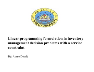
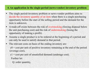
 It has been shown that how the optimisation problem with constraints in terms of
first and second moment of the demand distributions, has a dual program which is
a linear program with an infinite number of constraints.
 An idea is launched to replace the set of constraints by a large finite subset and
then to solve the so obtained linear program.
 The method assumes that integral constraints can be transformed into a sequence,
with increasing number of evaluation points, of optimisation problems and where
the integral is replaced by an infinite sum.
 Instead of evaluating the objective function on a continuous interval [low,high], the
functions are evaluated in a discrete number of points xi (i = 1. . .N).
 The assumption reflects the idea that if N→ ∞ the solution of the continuous
problem is found.
 It has been shown that how the optimisation problem with constraints in terms of
first and second moment of the demand distributions, has a dual program which is
a linear program with an infinite number of constraints.
 An idea is launched to replace the set of constraints by a large finite subset and
then to solve the so obtained linear program.
 The method assumes that integral constraints can be transformed into a sequence,
with increasing number of evaluation points, of optimisation problems and where
the integral is replaced by an infinite sum.
 Instead of evaluating the objective function on a continuous interval [low,high], the
functions are evaluated in a discrete number of points xi (i = 1. . .N).
 The assumption reflects the idea that if N→ ∞ the solution of the continuous
problem is found.
 It has been shown that how the optimisation problem with constraints in terms of
first and second moment of the demand distributions, has a dual program which is
a linear program with an infinite number of constraints.
 An idea is launched to replace the set of constraints by a large finite subset and
then to solve the so obtained linear program.
 The method assumes that integral constraints can be transformed into a sequence,
with increasing number of evaluation points, of optimisation problems and where
the integral is replaced by an infinite sum.
 Instead of evaluating the objective function on a continuous interval [low,high], the
functions are evaluated in a discrete number of points xi (i = 1. . .N).
 The assumption reflects the idea that if N→ ∞ the solution of the continuous
problem is found.
 It has been shown that how the optimisation problem with constraints in terms of
first and second moment of the demand distributions, has a dual program which is
a linear program with an infinite number of constraints.
 An idea is launched to replace the set of constraints by a large finite subset and
then to solve the so obtained linear program.
 The method assumes that integral constraints can be transformed into a sequence,
with increasing number of evaluation points, of optimisation problems and where
the integral is replaced by an infinite sum.
 Instead of evaluating the objective function on a continuous interval [low,high], the
functions are evaluated in a discrete number of points xi (i = 1. . .N).
 The assumption reflects the idea that if N→ ∞ the solution of the continuous
problem is found.

9. Cont….Cont….
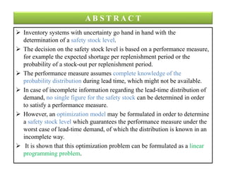
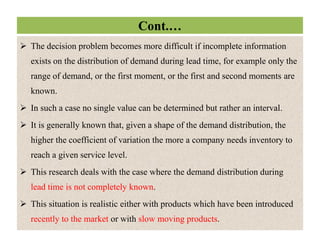
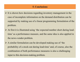
 This leads to an optimization problem, where:
t = the level of the inventory,
pi = the probability mass in point xi,
z1 = the expected value of X,
z2 = the absolute second moment of X,
z3 = the maximum allowed number of items short.
 The optimization problem might be formulated as:
 This leads to an optimization problem, where:
t = the level of the inventory,
pi = the probability mass in point xi,
z1 = the expected value of X,
z2 = the absolute second moment of X,
z3 = the maximum allowed number of items short.
 The optimization problem might be formulated as:
where (xi − t)+ stands for
max(xi − t, 0).
The decision variables in [P1] are t and pi (i = 1. . . N), where N represents the
number of discrete points which have been chosen in the experiment.

10. LINDO code for the illustrative exampleLINDO code for the illustrative example
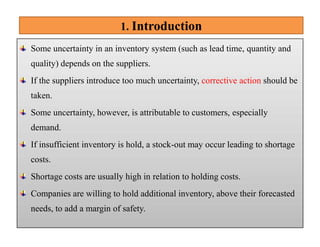
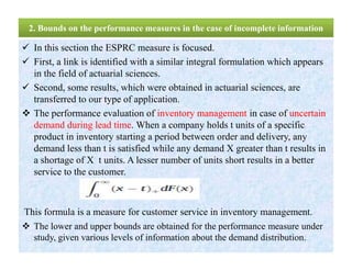
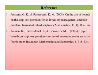
• With b0 = 50, the first and second moments in the interval [0, 50],
the following values l10 = 20 and l20 = 600 are used. The worked
out example, in LINDO code, is shown in Fig. 1. In this
approximation 10 intervals of equal length in the interval [0,50] are
chosen. Inclusion of both boundaries of the interval, the linear
program makes use of 11 xi-points.
Take for example the maximum number of units short W= 6. it can be
obtained that the lower bound for t equals t = 15. The linear program
in Fig. 1 leads to a minimum of t = 15, with probability mass in three
evaluation points x1 (X = 0), x4 (X = 15) and x11 (X = 50).
The respective probability masses are: p1 = 0.06667, p4 = 0.76195 and
p11 = 0.17143.
• With b0 = 50, the first and second moments in the interval [0, 50],
the following values l10 = 20 and l20 = 600 are used. The worked
out example, in LINDO code, is shown in Fig. 1. In this
approximation 10 intervals of equal length in the interval [0,50] are
chosen. Inclusion of both boundaries of the interval, the linear
program makes use of 11 xi-points.
Take for example the maximum number of units short W= 6. it can be
obtained that the lower bound for t equals t = 15. The linear program
in Fig. 1 leads to a minimum of t = 15, with probability mass in three
evaluation points x1 (X = 0), x4 (X = 15) and x11 (X = 50).
The respective probability masses are: p1 = 0.06667, p4 = 0.76195 and
p11 = 0.17143.

11. Cont…

12. 4. An application in the single-period (news-vendor) inventory problem
 The single period-inventory problem or news-vendor problem aims to
decide the inventory quantity of an item when there is a single purchasing
opportunity before the start of the selling period and the demand for the
item is unknown.
 A trade-off exists between the risk of overstocking (forcing disposal below
the unit purchasing cost) and the risk of understocking (losing the
opportunity of making a profit).
 Assume a single product is to be ordered at the beginning of a period and
can only be used to satisfy demand in that period.
 The relevant costs on basis of the ending inventory are:
c0 = cost per unit of positive inventory remaining at the end of the period
(overage cost),
c1 = cost per unit of unsatisfied demand (underage cost).
Further let:
Q: order quantity,
 The single period-inventory problem or news-vendor problem aims to
decide the inventory quantity of an item when there is a single purchasing
opportunity before the start of the selling period and the demand for the
item is unknown.
 A trade-off exists between the risk of overstocking (forcing disposal below
the unit purchasing cost) and the risk of understocking (losing the
opportunity of making a profit).
 Assume a single product is to be ordered at the beginning of a period and
can only be used to satisfy demand in that period.
 The relevant costs on basis of the ending inventory are:
c0 = cost per unit of positive inventory remaining at the end of the period
(overage cost),
c1 = cost per unit of unsatisfied demand (underage cost).
Further let:
Q: order quantity,

13. Cont..
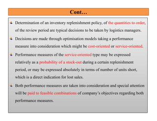
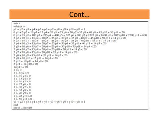
• D: random demand with a distribution F with density f defined on a
finite interval [a,b] with a≥0 and b > a.
• Define G(Q,D) as the total overage and underage cost incurred at the
end of period when Q units are ordered at the start of the period and
D is the demand. Then it follows that
 The expected cost G(Q) = E[G(Q,D)] can be calculated as: The expected cost G(Q) = E[G(Q,D)] can be calculated as:
 The news-vendor formulation also can be used to make decisions
in a profit framework.
 The objective function takes the form:

14. 5. Conclusions
 It is shown how decisions regarding inventory management in the
case of incomplete information on the demand distribution can be
supported by making use of a linear programming formulation of the
problem.
 At first it is illustrated using ‘the expected number short during lead-
time’ as a performance measure, and the same idea is also applied in
the news-vendor problem.
 A similar formulation can be developed making use of ‘the
probability of a stock-out during lead-time’ and, of course, also the
combination of both performance measures is also a challenging
input to this decision-making problem.
 It is shown how decisions regarding inventory management in the
case of incomplete information on the demand distribution can be
supported by making use of a linear programming formulation of the
problem.
 At first it is illustrated using ‘the expected number short during lead-
time’ as a performance measure, and the same idea is also applied in
the news-vendor problem.
 A similar formulation can be developed making use of ‘the
probability of a stock-out during lead-time’ and, of course, also the
combination of both performance measures is also a challenging
input to this decision-making problem.

15. Reference
1. Janssens, G. K., & Ramaekers, K. M. (2008). On the use of bounds
on the stop-loss premium for an inventory management decision
problem. Journal of Interdisciplinary Mathematics, 11(1), 115–126.
2. Janssen, K., Haezendonck, J., & Goovaerts, M. J. (1986). Upper
bounds on stop-loss premiums in case of known moments up to the
fourth order. Insurance: Mathematics and Economics, 5, 315–334.
1. Janssens, G. K., & Ramaekers, K. M. (2008). On the use of bounds
on the stop-loss premium for an inventory management decision
problem. Journal of Interdisciplinary Mathematics, 11(1), 115–126.
2. Janssen, K., Haezendonck, J., & Goovaerts, M. J. (1986). Upper
bounds on stop-loss premiums in case of known moments up to the
fourth order. Insurance: Mathematics and Economics, 5, 315–334.
1. Janssens, G. K., & Ramaekers, K. M. (2008). On the use of bounds
on the stop-loss premium for an inventory management decision
problem. Journal of Interdisciplinary Mathematics, 11(1), 115–126.
2. Janssen, K., Haezendonck, J., & Goovaerts, M. J. (1986). Upper
bounds on stop-loss premiums in case of known moments up to the
fourth order. Insurance: Mathematics and Economics, 5, 315–334.
1. Janssens, G. K., & Ramaekers, K. M. (2008). On the use of bounds
on the stop-loss premium for an inventory management decision
problem. Journal of Interdisciplinary Mathematics, 11(1), 115–126.
2. Janssen, K., Haezendonck, J., & Goovaerts, M. J. (1986). Upper
bounds on stop-loss premiums in case of known moments up to the
fourth order. Insurance: Mathematics and Economics, 5, 315–334.

16. THANK YOU FOR YOUR ATTTENTION !!!