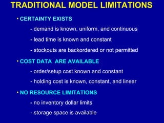
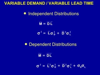
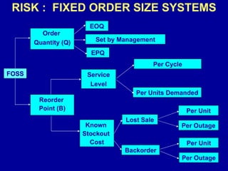
The document discusses inventory management models and concepts including: 1) Traditional inventory models make simplifying assumptions about demand, lead times, and costs that may not reflect reality. 2) Probabilistic models use statistical distributions to represent uncertain demand and lead times. Safety stock is calculated based on the probability of stockouts. 3) Service level goals can be set based on the probability of stockouts over an order cycle or per unit demanded. Imputed stockout costs are used to determine optimal reorder points.

1. TRADITIONAL MODEL LIMITATIONS CERTAINTY EXISTS - demand is known, uniform, and continuous - lead time is known and constant - stockouts are backordered or not permitted COST DATA ARE AVAILABLE - order/setup cost known and constant - holding cost is known, constant, and linear NO RESOURCE LIMITATIONS - no inventory dollar limits - storage space is available

2. WORKING AND SAFETY STOCK Safety Stock QUANTITY TIME B Q + S S Working Stock Working Stock

3. IDEAL INVENTORY MODEL B Q + S S QUANTITY Order Lot Order Lot Placed Received Placed Received Safety Stock Reorder Point Lead Time TIME

4. Q + S S Lead Time Lead Time Lead Time REALISTIC INVENTORY MODEL TIME B QUANTITY Stockout

5. SAFETY STOCK VERSUS SERVICE LEVEL .50 1.00 high SAFETY STOCK low SERVICE LEVEL (Probability of no stockouts)

6. STATISTICAL CONSIDERATIONS     max M 0 M ) M ( M P 0 M d ) M ( M f CONTINUOUS DISCRETE VARIABLE DISTRIBUTIONS DISTRIBUTIONS M                   max M 1 B M ) M ( P ) B M ( B M d ) M ( f ) B M ( Quantity Stockout Expected max M 1 B M ) M ( P B M d ) M ( f max M 0 M ) M ( P 2 ) M M ( 0 M d ) M ( f 2 ) M M ( Variance Demand Time Lead  2 E(M > B) P(M > B) B = reorder point in units. M = lead time demand in units (a random variable). f(M) = probability density function of lead time demand. P(M) = probability of a lead time demand of M units.  = standard deviation of lead time demand Demand Time Lead Mean Probability of a Stockout

7. PROBABILISTIC LEAD TIME DEMAND DEMAND DURING LEAD TIME (M) PROBABILITY OF A STOCKOUT, P(M>B) SAFETY STOCK REORDER POINT PROBABILITY P(M) 0 M B

8. NORMAL PROBABILITY DENSITY FUNCTION    2 ) ( 2 2 / 2 ) ( M M e M f    Lead Time Demand (M) M = 1 - F(B) = P(M >B) f(M) f(B) B Area   stockout a of probability B M P B F function distribution cumulative M d M f B F function density probability M f B = > = - = = =    ) ( ) ( 1 ) ( ) ( ) (

9. POISSON DISTRIBUTION LEAD TIME DEMAND (M) PROBABILITY P(M) 0.00 0.10 0.20 0.30 0.40 0 4 8 12 16 20 24 M=2 M=4 M=6 M=8 M=10 M=1 P(M) = M M e - M M!

10. NEGATIVE EXPONENTIAL DISTRIBUTION LEAD TIME DEMAND (M) PROBABILITY DENSITY F(M) 0 1/M f(M) = e  M/M M

11. NEGATIVE EXPONENTIAL DISTRIBUTION 0.0 0.5 1.0 1.5 2.0 2.5 0 2 4 6 8 10 12 LEAD TIME DEMAND (M) PROBABILITY DENSITY f(M) M=1 M=2 M=3 M=0.5 M=5 f(M) = e  M/M M

12. INDEPENDENT DEMAND : PROBABILISTIC MODELS LOT SIZE :  2CR / H REORDER POINT : B = M + S I. KNOWN STOCKOUT COST A. Obtain Lead Time Demand Distribution constant demand, constant lead time variable demand, constant lead time constant demand, variable lead time variable demand, variable lead time B. Stockout Cost backorder cost / unit lost sale cost / unit II. SERVICE LEVEL A. Service per Order Cycle

13. Demand Probability Demand Probability Lead time Probability first week second week demand (col. 2)(col. 4) (D) P(D) (D) P(D) (M) P(M) 1 0.60 1 0.60 2 0.36 3 0.30 4 0.18 4 0.10 5 0.06 3 0.30 1 0.60 4 0.18 3 0.30 6 0.09 4 0.10 7 0.03 4 0.10 1 0.60 5 0.06 3 0.30 7 0.03 4 0.10 8 0.01 CONVOLUTIONS (variable demand/week and constant lead time of 2 weeks)

14. Lead time demand (M) Probability P(M) 0 0 1 0 2 0.36 3 0 4 0.36 5 0.12 6 0.09 7 0.06 8 0.01 1.00

15. INVENTORY RISK ( VARIABLE DEMAND, CONSTANT LEAD TIME ) J S 0 W Q + S -W B TIME QUANTITY L P(M>B) Q = order quantity B = reorder point L = lead time S = safety stock B - S = expected lead time demand B - J = minimum lead time demand B + W = maximum lead time demand P(M>B) = probability of a stockout J

16. SAFETY STOCK : BACKORDERING M B S M d M f M M d M f B M d M f M B S - =           ) ( ) ( ) ( ) ( ) ( ) ( ) ( 0 0 0

17. BACKORDERING Cost Stockout Cost Holding TC S + = B M P Q AR H dB dTC S     0 ) ( B M E Q AR H M B     ) ( ) (  M d M f B M Q AR SH     ) ( ) ( ) ( B AR HR s P B M P    ) ( ) (

18. TC s = (B - M)H + E(M > B) = B = 67 E(M > B) = = (68- 67).08 + (69- 67).03 + (70- 67).01 = .17 units TC s = (67- 65)(2)(.30) + = 1.20 + 2.04 = $3.24 B = 68 E(M > B) = = (69- 68).03 + (70- 68).01 = .05 units TC s = (68- 65)(2)(.30) + = 1.80 + 0.60 = $2.40 AR E(M>B) Q 2(3600)(.05) 600 2(3600)(.17) 600  + = - 70 1 68 ) ( ) 68 ( M M P M     max 1 ) ( ) ( M B M M P B M  + = - 70 1 67 ) ( ) 67 ( M M P M

19. B = 69 E(M > B) = = (70- 69).01 = .01 units TC s = (69- 65)(2)(.30) + = 2.40 + 0.12 = $2.52  + = - 70 1 69 ) ( ) 69 ( M M P M 2(3600)(.01) 600 Therefore, the lowest cost reorder point is 68 units with an expected annual cost of safety stock of $2.40.

20. SAFETY STOCK : LOST SALES ) ( ) ( 0 M d M f M B S B - =  ) ( B M E M B S > + - = ) ( ) ( M d M f B M M B B - + - =   ) ( ) ( ) ( ) ( 0 M d M f M B M d M f M B B - - - =    

21. LOST SALES Cost Stockout Holding Cost TC S  = HQ AR HQ s P B M P  = =  ) ( ) ( B M P H Q AR H dB dTC S =          = 0 ) (   B M E Q AR H B M E M B      = ) ( ) ( M d M f B M Q AR SH B - + =   ) ( ) ( B M E H Q AR H M B           = ) ( ) (

22. INVENTORY RISK (CONSTANT DEMAND, VARIABLE LEAD TIME) Q + S S B L m L QUANTITY TIME P(M > B) 0 L = expected lead time P(M > B) = probability of a stockout B - S = expected lead time demand Q = order quantity B = reorder point S = safety stock L m = maximum lead time

23. J S 0 Q + S - W B QUANTITY L m INVENTORY RISK (VARIABLE DEMAND, VARIABLE LEAD TIME) L TIME P(M >B) P(M > B) = probability of a stockout B - S = expected lead time demand B + W = maximum lead time demand Q = order quantity B = reorder point S = safety stock L = expected lead time L m = maximum lead time B - J = minimum lead time demand

24. VARIABLE DEMAND / VARIABLE LEAD TIME L D D L      2 2 2 2 Independent Distributions L D M  L D D D L L D M          2 2 2 2 2 Dependent Distributions L

25. SERVICE PER ORDER CYCLE c c SL B M P B M P cycles order of no total stockout a with cycles of no SL  =  >  =  = 1 ) ( ) ( 1 . . 1

26. IMPUTED STOCKOUT COSTS ) ( ) ( / cost B M P R HQ A AR HQ B M P unit Backorder        ) ( ) ( 1 ) ( / B M P R B M P HQ A HQ AR HQ B M P unit sales cost Lost        

27. SAFETY STOCK : 1 WEEK TIME SUPPLY (Normal Distribution : Lead Time = 4 weeks) Weekly Demand Safety Stock D  D 1000 100 1000 5.00 0 1000 200 1000 2.50 0.0062 1000 300 1000 1.67 0.0480 1000 400 1000 1.25 0.1057 1000 500 1000 1.00 0.1587 4 1000 D S Z     S P(M>B)

28. PROBABILISTIC LOGIC Service Levels Service/units demanded, E(M>B) = Q(1 - SL U ) E(M>B) =  E(Z) Convolution over lead time Multiply dist. by demand, M = DL,  = D  L Analytical Combination / Monte Carlo simulation Service/cycle, P(M>B) = 1 - SL c Variable demand, variable lead time Variable demand, constant lead time Constant demand, variable lead time Lost Sale, P(M>B) = HQ / (AR+HQ) Backordering, P(M>B) = HQ / AR Lead time demand distribution ? Known stockout costs ? No Yes Yes No Start

29. RISK : FIXED ORDER SIZE SYSTEMS FOSS Order Quantity (Q) Reorder Point (B) Set by Management EOQ EPQ Service Level Per Cycle Per Units Demanded Known Stockout Cost Lost Sale Backorder Per Outage Per Unit Per Outage Per Unit