Downloaded 30 times

![ Then the probability of a demand in any period is
1/ET, so we can forecast demand from : Forecast
Demand = ED/ET
If we know the shortage cost we can balance this
against holding cost and calculate an optimal value
for A, the amount of stock that minimizes the
expected total cost . Alternatively , we can look at
the service level , with Service level = 1-
prob(shortage)
=1-[prob(there is demand)xProb(demand>A)]](https://image.slidesharecdn.com/inventoryppt-141024004832-conversion-gate02/75/Inventory-control-and-management-19-2048.jpg)
![ Example : Mean time between demands for spare part
is 5 weeks, and the mean demand size is 10 units . If
the demand size is normally dist. With Std. deviation of
3 units , what stock level would give a 95% service
level?
Ans: we know that service level =
1-[Prob(there is demand)xProb(demand>A)] and we
want Prob(there is demand)xProb(demand>A)=.05
but Prob(there is demand) = 1/5 so Prob(demand>A)
= .05/2 =.25 for the norm. dist. This equals to 0.67 s.d
giving A=ED+Z.σ=10+0.67x3 =12units . This ans
makes assumptions but its reasonable](https://image.slidesharecdn.com/inventoryppt-141024004832-conversion-gate02/75/Inventory-control-and-management-21-2048.jpg)
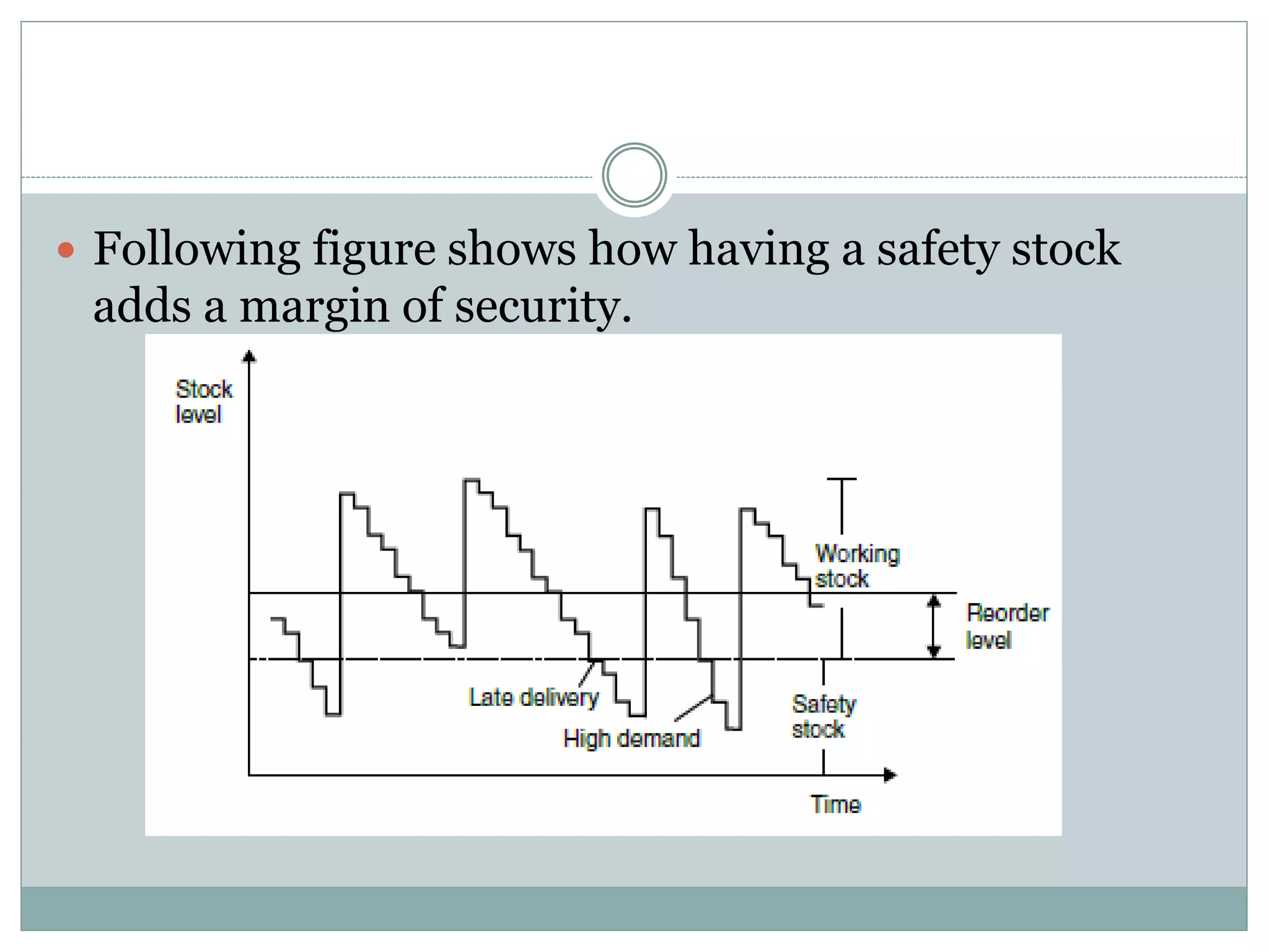
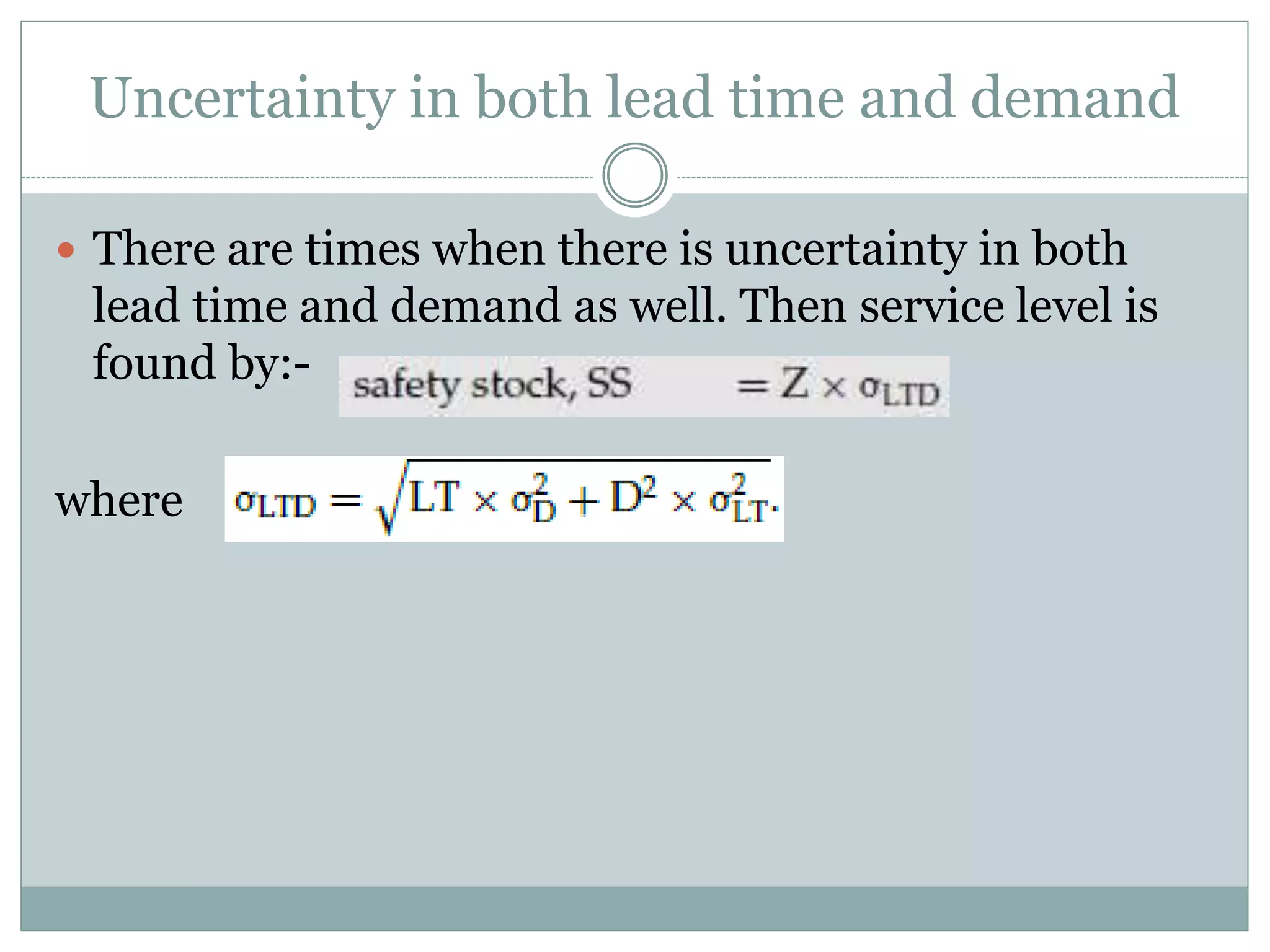
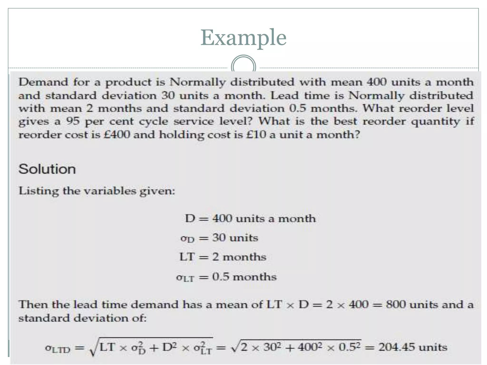
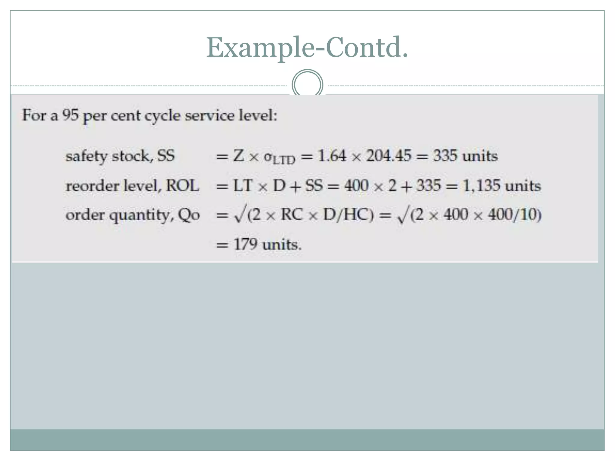

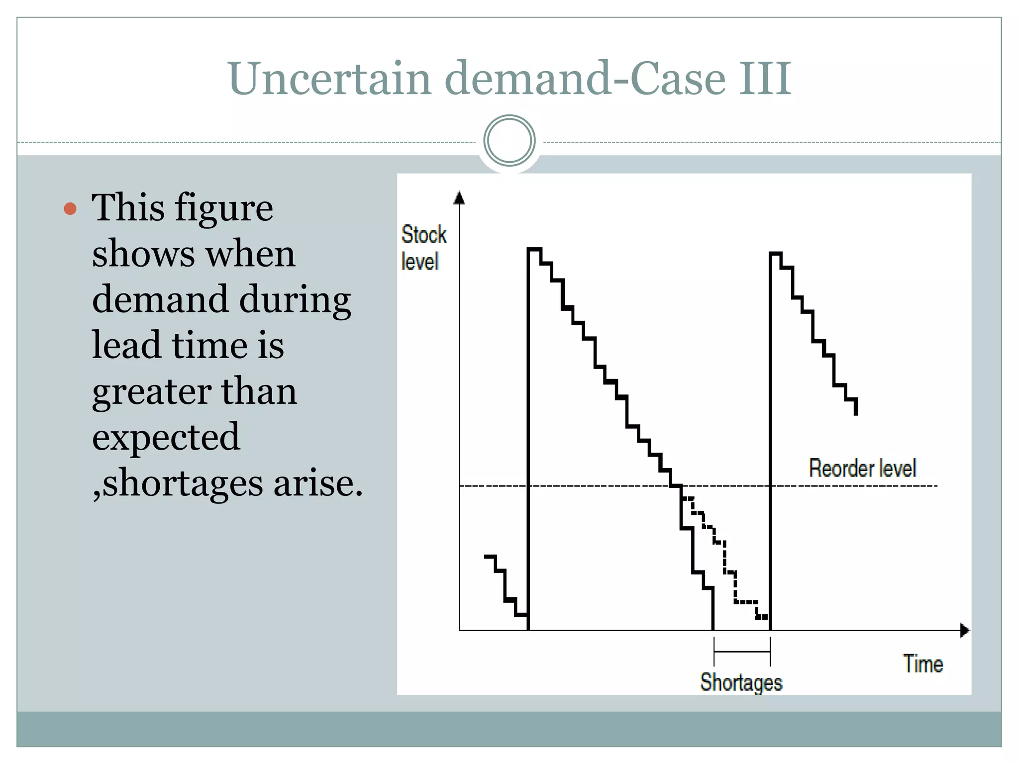
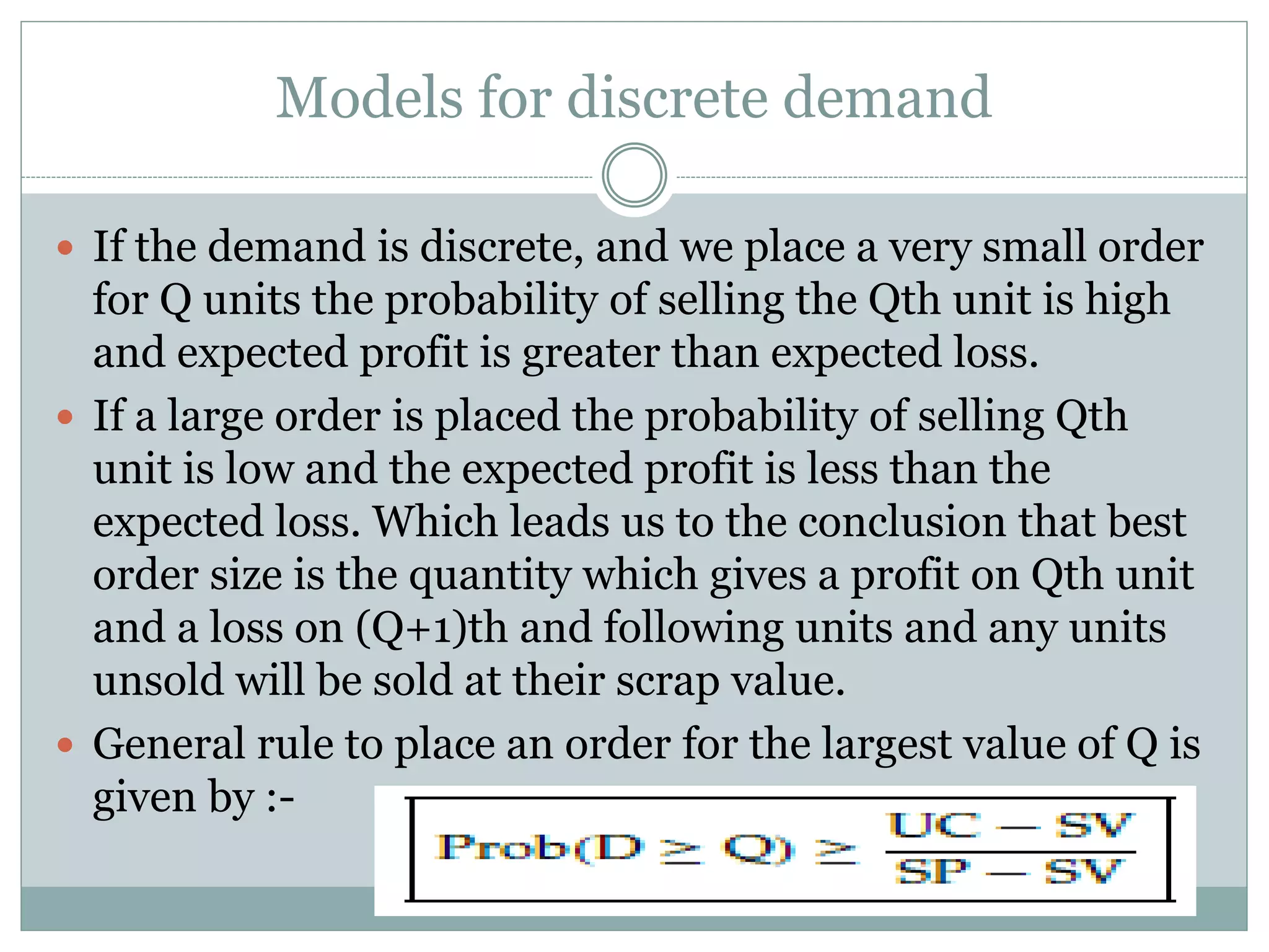
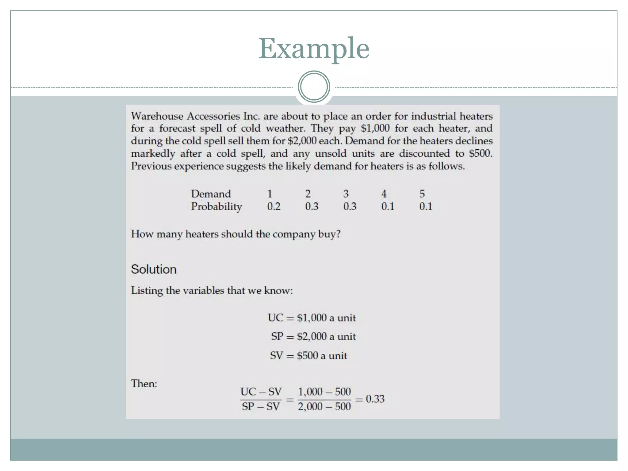
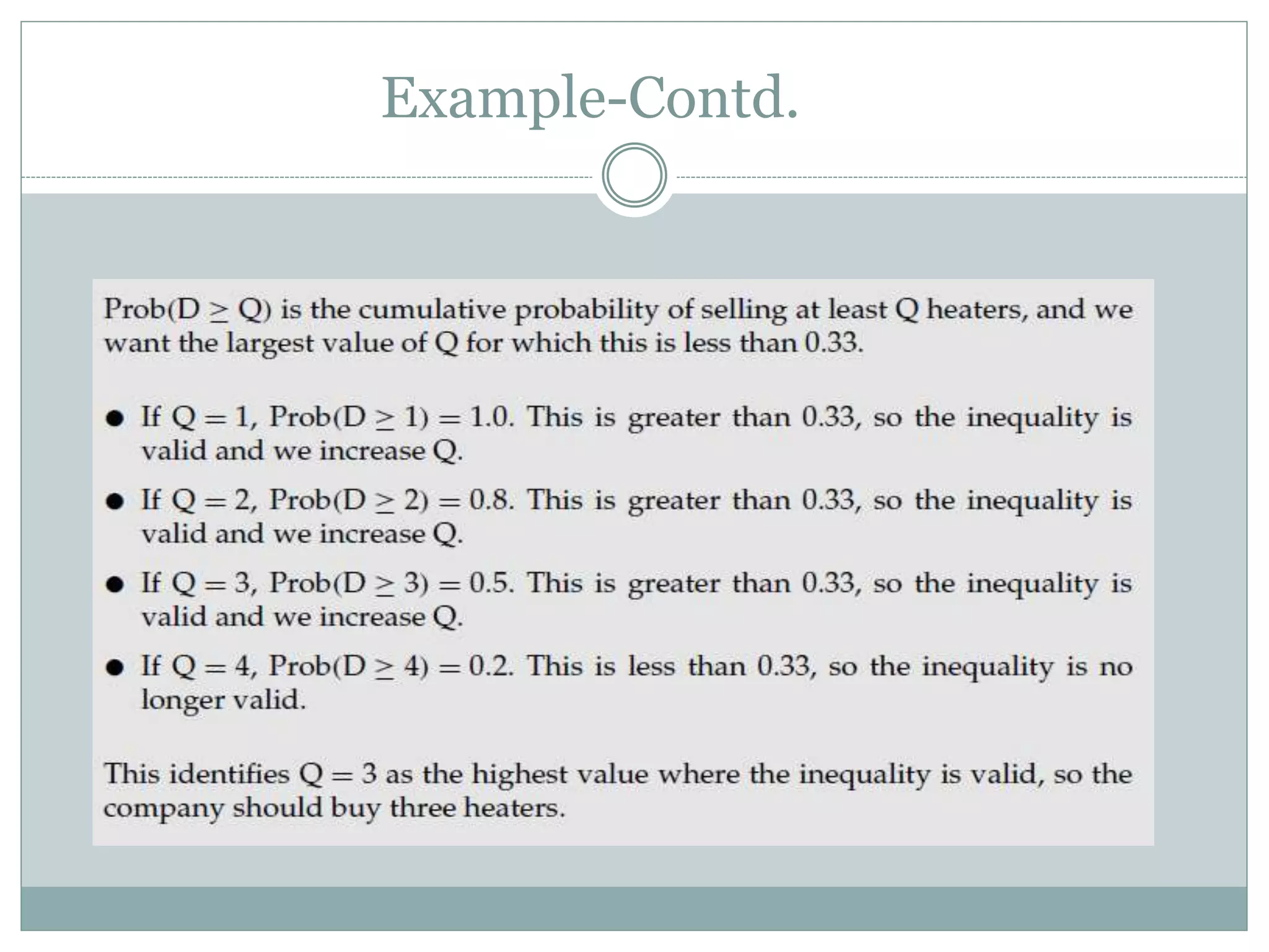
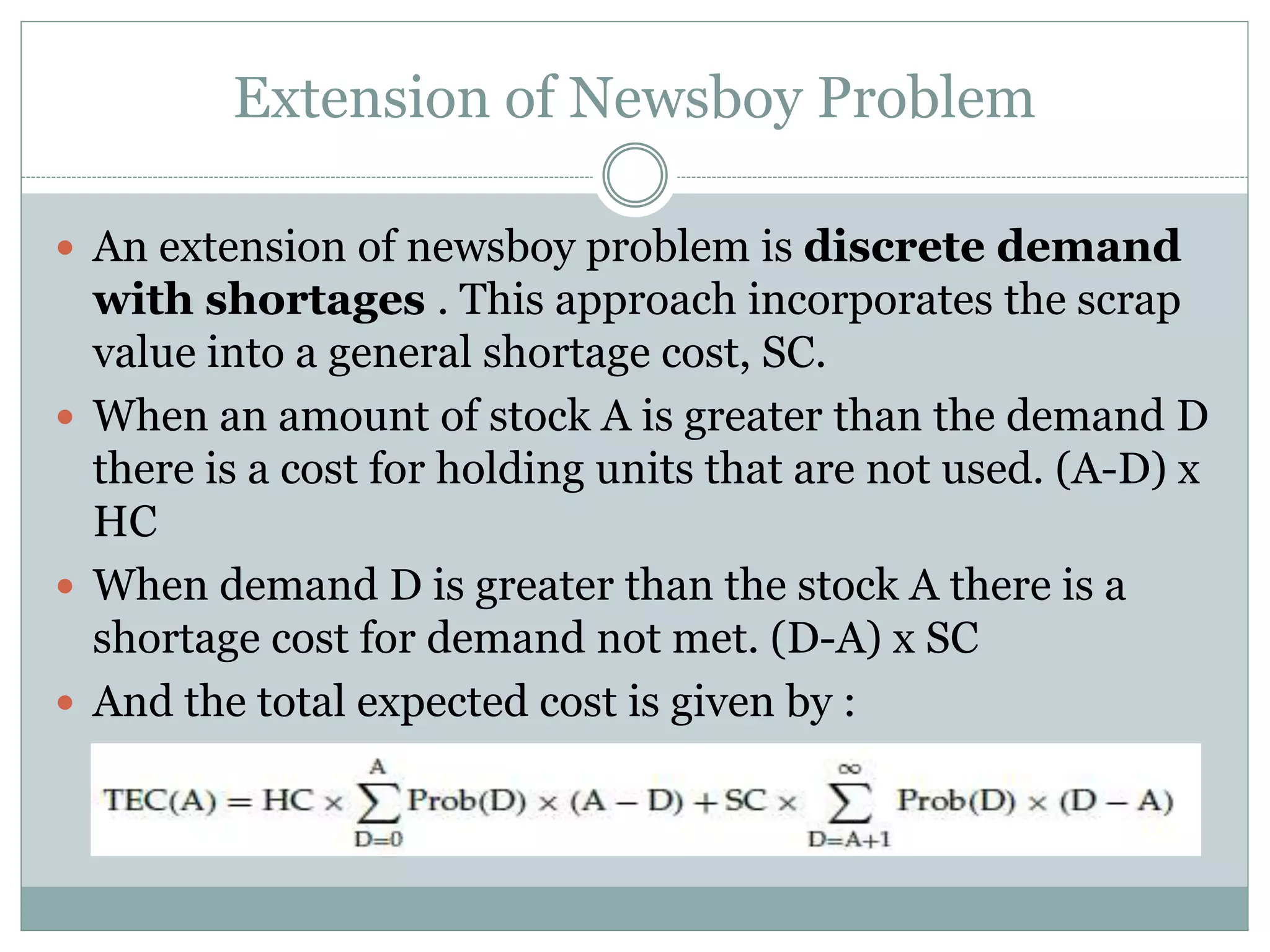
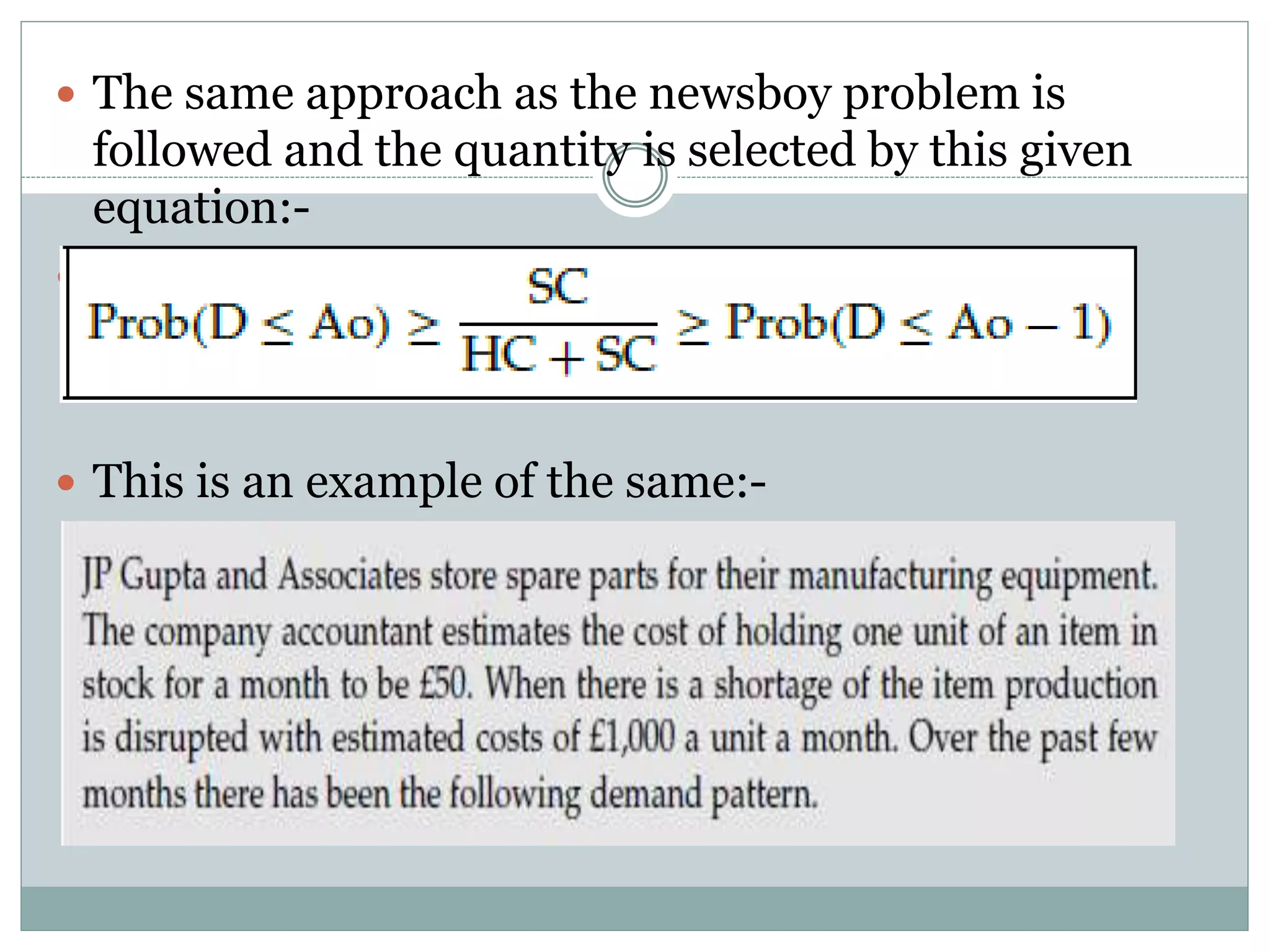
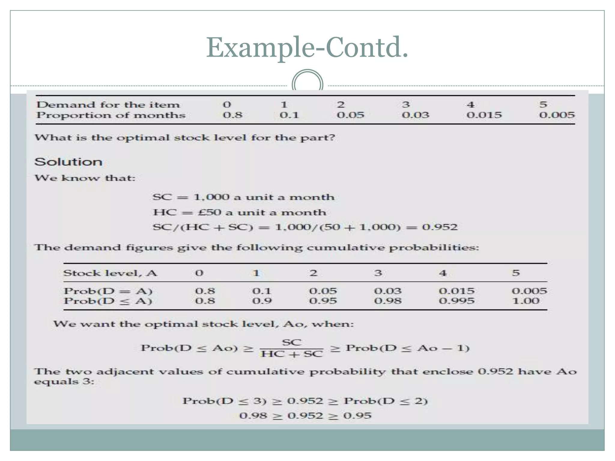
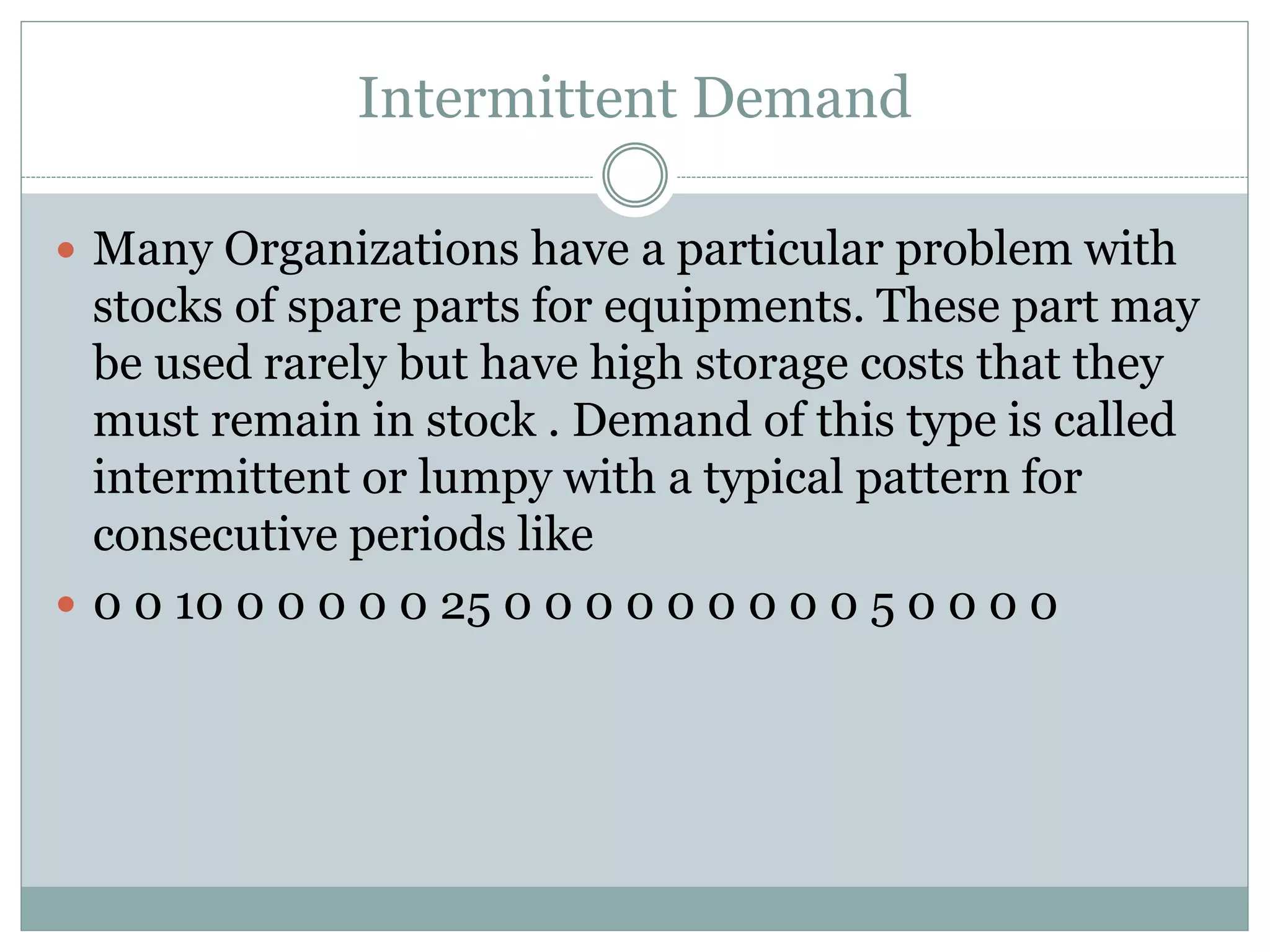
The document discusses various models for managing inventory and dealing with uncertainty in demand, costs, lead times, and other factors. It describes how uncertainty can be classified as unknown, known, or uncertain and probabilistic models can handle uncertain situations. Different cases of uncertain demand are illustrated, and models for discrete demand, the newsboy problem, shortages, intermittent demand, service level, and target stock levels are explained. Examples are provided to demonstrate how to determine optimal order quantities, safety stocks, reorder levels, and target inventory levels given uncertainty in demand and lead times.


