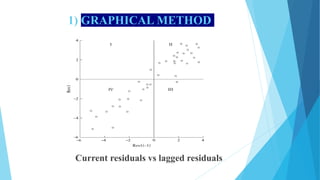
PANDIT JAWAHARLAL NEHRU COLLEGE OF AGRICULTURE AND RESEARCH INSTITUTE
DEPARTMENT OF AGRICULTURAL ECONOMICS AND EXTENTION
AEC 507 ECONOMETRICS (2+1)
COURSE TEACHER: Dr. L.UMAMAHESWARI
TOPIC: AUTOCORRELATION
PRESENTED BY
T.PRIYADHARSHAN
22PGA103
AUTOCORRELATION
 The term autocorrelation may be defined as “correlation
between members of series of observations ordered in time [as
in time series data]”.
 In the regression context, the classical linear regression model
assumes that such autocorrelation does not exist in the
disturbances ui. Symbolically,
E(ui, uj ) = 0, i ≠ j (or)
Cov(ui, uj / xi, xj) = 0, means the disturbance ui and uj are
uncorrelated.
AUTOCORRELATION
 The term autocorrelation or serial correlation means the error
term in one time period is positively or negatively
correlated with the error term in any other time period.
This is common in time-series analysis.
The possible patterns
 Inertia
 A salient feature of most economic time series is inertia or sluggishness.
 Time series data such as GNP, price index, production, employment and
unemployment exhibit cycles.
 Therefore in regressions involving time-series data, successive observations are
likely to be interdependent.
Cause for serial correlation
Specification bias
a) Excluded variable case
When residuals exhibit a pattern as in figures a to d, is
case of excluded variable specification bias and the
inclusion such variables removes the correlation patterns
observed among the variables.
(1)
where, Y= Quantity of beef demanded
X2= Price of beef
X3= Consumer income
X4= Price of pork
t= time
Suppose we estimate the regression
(2)
(3)
As X4 affects consumption of beef, v will reflect a systematic pattern,
thus creating autocorrelation.
b) Incorrect functional form
Suppose instead of the correct model
(4)
we fit the model
(5)
SPECIFICATION BIAS: INCORRECT
FUNCTIONAL FORM
 Between points A and B, linear marginal cost curve
will overestimate the true MC and beyond these points
it will underestimate the true MC. Here vi reflects
autocorrelation because of incorrect functional form.
 Exclusion of lagged variables
In the time-series regression of consumption expenditure on
income, consumption expenditure in the current period depend
among other things on consumption of previous period.
If the lagged term is deleted, the resulting error will reflect a
systematic pattern due to the influence of lagged consumption on
current consumption.
OLS Estimators and their Variance
in the presence of autocorrelation
 The OLS consequences are still unbiased and consistent and
asymptotically normally distributed.
 The OLS estimators will be inefficient and therefore no longer
BLUE.
 The estimated variances of the regression coefficients will be
biased and inconsistent, and therefore hypothesis testing is no
longer valid. In most of the cases, the R2 will be overestimated
and the t-statistics will tend to be higher.
DETECTING AUTOCORRELATION
 The Graphical Test
 The Runs Test
 The Durbin Watson Test
 The Breusch-Godfrey Test
1) GRAPHICAL METHOD
Current residuals vs lagged residuals
 In this graph, u^ is plotted against u^
t-1, that is, plot the
residuals at time t against their value at time (t-1), (i.e),
current residuals VS lagged residuals. As this figure
reveals, most of the residuals are bunched in the second
(northeast) and the fourth (southwest) quadrants,
suggesting a strong positive correlation in the residuals.
Standardized residuals VS time
 Standardized residuals versus time, which is u^
t /√σ^2,
(i.e), u^
t is divided by the residuals SE of estimate.
 As it is a random sequence without any pattern,
autocorrelation is not present in the data.
 The graphical method we have just discussed, although
powerful and suggestive, is subjective or qualitative in
nature. But there are several quantitative tests that can be
used to supplement the purely qualitative approach.
2) THE RUNS TEST
 The runs test is also called as Geary test.
 It is a non- parametric test.
 A run is defined as an uninterrupted sequence of one
symbol or attribute, such as positive or negative.
 Note down the signs (positive or negative) of the
residuals.
 Length of the run is the number of elements in the run.
 If there are two many runs, it means that ut’s change
sign frequently indicating negative autocorrelation.
 Similarly, if there are too few runs, they may suggest
positive autocorrelation.
 Now let,
N = Total no of observation N1+N2
N1= No of + symbols(i.e., + residuals)
N2= No of - symbols(i.e., - residuals)
R = No of runs
 Then under the null hypothesis that the successive
outcomes (here, residuals) are independent, and
assuming that N1> 10 and N2> 10, the number of runs is
(asymptotically) normally distributed with
 Note: N = N₁ + N₂. If the null hypothesis of randomness
is sustainable, following the proper ties of the normal
distribution, we should expect that
 That is, the probability is 95 percent that the preceding
interval will include R.
 Decision Rule:
Do not reject the null hypothesis of randomness with
95% confidence if R, the number of runs, lies in the
preceding confidence interval.
Reject the null hypothesis if the estimated R lies
outside these limits.
3) Durbin-Watson d test
 It is a popular method and Durbin-Watson d statistic
is given
(1)
 Thus ‘d’ is simply the ratio of the sum of squared
difference in successive residuals to the RSS.
Applying (a+b)2 formula gives,
( 2 (2)
 Since ∑u^2
t and ∑u^2
t-1 differ in only one observation,
they are approximately equal. Therefore, setting
 d may be written as
(3)
(4)
d ≈ 2(1 − ρˆ) (5)
As −1 ≤ ρ ≤ 1, in equation (5) implies that
0 ≤ d ≤ 4 (6)
from equation (5), if ρ^ = 0, d = 2, there is no autocorrelation
ρ^ = +1, d = 0, there is positive autocorrelation in the residuals
ρ^ = -1, d = 4, there is negative autocorrelation in the residuals
Therefore, closer d to 0, greater the evidence of positive serial correlation
d to 4, greater the evidence of negative serial correlation
d to 2, there is no first order autocorrelation, either positive or negative.
Durbin-Watson ‘d’ statistic
 H0 : No positive autocorrelation
 H0* : No negative autocorrelation
Durbin-Watson ‘d’ test: Decision rules
D-W d test:
 Run OLS regression & obtain residuals ut
 Compute ‘d’
 For the given sample size & explanatory variables, find
out the critical dL and du values.
 Follow the decision rule
Limitation of d test
If ‘d’ falls in the indecisive zone (or) region of ignorance,
one cannot conclude whether autocorrelation does (or)
does not exist.
4) The Breusch-Godfrey (BG) Test
 It is also called as Lagrange Multiplier test (LM Test).
 To avoid some of the drawbacks of the Durbin–Watson d test of
autocorrelation, statisticians Breusch and Godfrey have developed a
test of autocorrelation that allows for lagged values of the regressand
and higher-order autoregressive schemes, such as AR(1), AR(2), etc.
The BG Test:
Consider a two- variable regression model:
let (1)
Assume error term ut follows the pth order autoregressive scheme
AR(p) as follows:
(2)
Where, εt is a white noise error term
(3)
(i.e), there is no serial correlation of any order.
The BG test involves the following steps:
1. Estimate by OLS and obtain the residuals u^
t.
2. Regress u^t on original xt and u^
t-1 , u^
t-2 ………. u^
t-p (which
are the lagged values of the estimated residuals in step 1). Thus
if p=4, we will introduce four lagged values of the residuals as
additional regressors in the model.
Run the regression,
(4)
and obtain R2 from this auxiliary regression.
3. If the sample size is large, BG have shown that
(5)
 That is, asymptotically, n-p times the R2 value obtained
from the auxiliary regression (2) follows the chi-square
distribution with p.d.f. if (n-p) R2 exceeds the critical chi-
square value at the chosen level of significance, we reject
the null hypothesis, and there is autocorrelation in the data.
 If in equation (2) ρ=1, meaning first-order autoregression,
then the BG test is known as Durbin’s M Test.
(1) Generalized Least Squares method
Let us assume that ut follows the first order autoregressive
scheme (AR1),
(1)
ρ is called first order coefficient of autocorrelation (or) coefficient
of autocorrelation of lag 1 (or) coefficient of autocorrelation.
(2)
 When ρ is known
if eq (2) holds true at time t, it also holds true at t-1
so, (3)
REMEDIAL MEASURES WHEN AUTOCORRELATION IS FOUND
Multiplying by ρ on both sides, we obtain
(4)
eq (2) - (4) gives,
(5)
Eqtn (5) is the generalized difference equation & can be written as
(6)
where
To avoid the loss of one observation, the first observation on Y and X is
transformed as follows:
Y1√ 1- ρ2 and X1 √1-ρ2. This transformation is known as the Prais-
Winsten transformation.
 As error term satisfied OLS assumptions, we can apply
OLS to the transformed variables Y* and X* and obtain
estimators with optimum properties, i.e. BLUE
 GLS is nothing but OLS applied to the transformed
model that satisfies the classical assumptions.
 When ρ is not known
As ρ is rarely known in practice, generalized
difference regression is difficult to run and therefore
alternative methods are discussed below:
(a) The first difference method
If ρ = +1, the generalized difference equation (5) reduces the
first difference equation as
(7)
An important feature of the first difference model is that
there is no intercept term in it. Hence to run (7), the
regression through the origin model have to be used.
 If ρ = -1, the generalized difference equation becomes
 Yt + Yt-1 = 2 β1 + β2(Xt+Xt-1) + εt
 Yt + Yt-1 / 2 = β1 + β2(Xt+Xt-1) /2 + εt /2
 This model is known as Moving Average Regression
Model as we are regressing the value of one moving
average on another
(3) Based on Durbin- Watson d statistics
If we cannot use the first difference transformation because ρ
is not sufficiently close to unity, we have an easy method of
estimating it from the relationship between d and ρ established, from
which we can estimate ρ as follows:
 d = 2(1- ρˆ)
 (1- ρˆ) = d/2
 ρˆ = 1- d/2
(4) Durbin’s two step procedure of estimating ρ:
1. Estimate Yt on Xt, Xt-1 and Yt-1
Yt = β1 (1-ρ) + β2 Xt - ρ β2 Xt-1 + ρ Yt-1 + ԑt
and treat the estimated value of the regression coefficient of Yt-1 as an
estimate of ρ.
2. Having obtained ρ^ , transform the variables as
Yt* = (Yt - ρ^Y t-1) and Xt* = (Xt - ρ^Xt-1) and run the OLS
regression on transformed variables to obtain estimate of parameters.
REFERENCE:
 Basic Econometrics- Sixth edition- Damodar N
Gujarathi, Dawn C Porter, Manorajan Pal
THANK YOU

autocorrelation.pptx

  • 1.
    PANDIT JAWAHARLAL NEHRUCOLLEGE OF AGRICULTURE AND RESEARCH INSTITUTE DEPARTMENT OF AGRICULTURAL ECONOMICS AND EXTENTION AEC 507 ECONOMETRICS (2+1) COURSE TEACHER: Dr. L.UMAMAHESWARI TOPIC: AUTOCORRELATION PRESENTED BY T.PRIYADHARSHAN 22PGA103
  • 2.
    AUTOCORRELATION  The termautocorrelation may be defined as “correlation between members of series of observations ordered in time [as in time series data]”.  In the regression context, the classical linear regression model assumes that such autocorrelation does not exist in the disturbances ui. Symbolically, E(ui, uj ) = 0, i ≠ j (or) Cov(ui, uj / xi, xj) = 0, means the disturbance ui and uj are uncorrelated.
  • 3.
    AUTOCORRELATION  The termautocorrelation or serial correlation means the error term in one time period is positively or negatively correlated with the error term in any other time period. This is common in time-series analysis.
  • 4.
  • 6.
     Inertia  Asalient feature of most economic time series is inertia or sluggishness.  Time series data such as GNP, price index, production, employment and unemployment exhibit cycles.  Therefore in regressions involving time-series data, successive observations are likely to be interdependent. Cause for serial correlation
  • 7.
    Specification bias a) Excludedvariable case When residuals exhibit a pattern as in figures a to d, is case of excluded variable specification bias and the inclusion such variables removes the correlation patterns observed among the variables.
  • 8.
    (1) where, Y= Quantityof beef demanded X2= Price of beef X3= Consumer income X4= Price of pork t= time Suppose we estimate the regression (2) (3) As X4 affects consumption of beef, v will reflect a systematic pattern, thus creating autocorrelation.
  • 9.
    b) Incorrect functionalform Suppose instead of the correct model (4) we fit the model (5)
  • 10.
  • 11.
     Between pointsA and B, linear marginal cost curve will overestimate the true MC and beyond these points it will underestimate the true MC. Here vi reflects autocorrelation because of incorrect functional form.
  • 12.
     Exclusion oflagged variables In the time-series regression of consumption expenditure on income, consumption expenditure in the current period depend among other things on consumption of previous period. If the lagged term is deleted, the resulting error will reflect a systematic pattern due to the influence of lagged consumption on current consumption.
  • 13.
    OLS Estimators andtheir Variance in the presence of autocorrelation  The OLS consequences are still unbiased and consistent and asymptotically normally distributed.  The OLS estimators will be inefficient and therefore no longer BLUE.  The estimated variances of the regression coefficients will be biased and inconsistent, and therefore hypothesis testing is no longer valid. In most of the cases, the R2 will be overestimated and the t-statistics will tend to be higher.
  • 14.
    DETECTING AUTOCORRELATION  TheGraphical Test  The Runs Test  The Durbin Watson Test  The Breusch-Godfrey Test
  • 15.
    1) GRAPHICAL METHOD Currentresiduals vs lagged residuals
  • 16.
     In thisgraph, u^ is plotted against u^ t-1, that is, plot the residuals at time t against their value at time (t-1), (i.e), current residuals VS lagged residuals. As this figure reveals, most of the residuals are bunched in the second (northeast) and the fourth (southwest) quadrants, suggesting a strong positive correlation in the residuals.
  • 17.
  • 18.
     Standardized residualsversus time, which is u^ t /√σ^2, (i.e), u^ t is divided by the residuals SE of estimate.  As it is a random sequence without any pattern, autocorrelation is not present in the data.  The graphical method we have just discussed, although powerful and suggestive, is subjective or qualitative in nature. But there are several quantitative tests that can be used to supplement the purely qualitative approach.
  • 19.
    2) THE RUNSTEST  The runs test is also called as Geary test.  It is a non- parametric test.  A run is defined as an uninterrupted sequence of one symbol or attribute, such as positive or negative.  Note down the signs (positive or negative) of the residuals.
  • 20.
     Length ofthe run is the number of elements in the run.  If there are two many runs, it means that ut’s change sign frequently indicating negative autocorrelation.  Similarly, if there are too few runs, they may suggest positive autocorrelation.
  • 21.
     Now let, N= Total no of observation N1+N2 N1= No of + symbols(i.e., + residuals) N2= No of - symbols(i.e., - residuals) R = No of runs
  • 22.
     Then underthe null hypothesis that the successive outcomes (here, residuals) are independent, and assuming that N1> 10 and N2> 10, the number of runs is (asymptotically) normally distributed with
  • 23.
     Note: N= N₁ + N₂. If the null hypothesis of randomness is sustainable, following the proper ties of the normal distribution, we should expect that  That is, the probability is 95 percent that the preceding interval will include R.
  • 24.
     Decision Rule: Donot reject the null hypothesis of randomness with 95% confidence if R, the number of runs, lies in the preceding confidence interval. Reject the null hypothesis if the estimated R lies outside these limits.
  • 25.
    3) Durbin-Watson dtest  It is a popular method and Durbin-Watson d statistic is given (1)  Thus ‘d’ is simply the ratio of the sum of squared difference in successive residuals to the RSS. Applying (a+b)2 formula gives, ( 2 (2)
  • 26.
     Since ∑u^2 tand ∑u^2 t-1 differ in only one observation, they are approximately equal. Therefore, setting  d may be written as (3)
  • 27.
    (4) d ≈ 2(1− ρˆ) (5) As −1 ≤ ρ ≤ 1, in equation (5) implies that 0 ≤ d ≤ 4 (6) from equation (5), if ρ^ = 0, d = 2, there is no autocorrelation ρ^ = +1, d = 0, there is positive autocorrelation in the residuals ρ^ = -1, d = 4, there is negative autocorrelation in the residuals Therefore, closer d to 0, greater the evidence of positive serial correlation d to 4, greater the evidence of negative serial correlation d to 2, there is no first order autocorrelation, either positive or negative.
  • 28.
  • 29.
     H0 :No positive autocorrelation  H0* : No negative autocorrelation Durbin-Watson ‘d’ test: Decision rules
  • 30.
    D-W d test: Run OLS regression & obtain residuals ut  Compute ‘d’  For the given sample size & explanatory variables, find out the critical dL and du values.  Follow the decision rule Limitation of d test If ‘d’ falls in the indecisive zone (or) region of ignorance, one cannot conclude whether autocorrelation does (or) does not exist.
  • 31.
    4) The Breusch-Godfrey(BG) Test  It is also called as Lagrange Multiplier test (LM Test).  To avoid some of the drawbacks of the Durbin–Watson d test of autocorrelation, statisticians Breusch and Godfrey have developed a test of autocorrelation that allows for lagged values of the regressand and higher-order autoregressive schemes, such as AR(1), AR(2), etc.
  • 32.
    The BG Test: Considera two- variable regression model: let (1) Assume error term ut follows the pth order autoregressive scheme AR(p) as follows: (2) Where, εt is a white noise error term (3) (i.e), there is no serial correlation of any order.
  • 33.
    The BG testinvolves the following steps: 1. Estimate by OLS and obtain the residuals u^ t. 2. Regress u^t on original xt and u^ t-1 , u^ t-2 ………. u^ t-p (which are the lagged values of the estimated residuals in step 1). Thus if p=4, we will introduce four lagged values of the residuals as additional regressors in the model. Run the regression, (4) and obtain R2 from this auxiliary regression. 3. If the sample size is large, BG have shown that (5)
  • 34.
     That is,asymptotically, n-p times the R2 value obtained from the auxiliary regression (2) follows the chi-square distribution with p.d.f. if (n-p) R2 exceeds the critical chi- square value at the chosen level of significance, we reject the null hypothesis, and there is autocorrelation in the data.  If in equation (2) ρ=1, meaning first-order autoregression, then the BG test is known as Durbin’s M Test.
  • 35.
    (1) Generalized LeastSquares method Let us assume that ut follows the first order autoregressive scheme (AR1), (1) ρ is called first order coefficient of autocorrelation (or) coefficient of autocorrelation of lag 1 (or) coefficient of autocorrelation. (2)  When ρ is known if eq (2) holds true at time t, it also holds true at t-1 so, (3) REMEDIAL MEASURES WHEN AUTOCORRELATION IS FOUND
  • 36.
    Multiplying by ρon both sides, we obtain (4) eq (2) - (4) gives, (5) Eqtn (5) is the generalized difference equation & can be written as (6) where To avoid the loss of one observation, the first observation on Y and X is transformed as follows: Y1√ 1- ρ2 and X1 √1-ρ2. This transformation is known as the Prais- Winsten transformation.
  • 37.
     As errorterm satisfied OLS assumptions, we can apply OLS to the transformed variables Y* and X* and obtain estimators with optimum properties, i.e. BLUE  GLS is nothing but OLS applied to the transformed model that satisfies the classical assumptions.
  • 38.
     When ρis not known As ρ is rarely known in practice, generalized difference regression is difficult to run and therefore alternative methods are discussed below: (a) The first difference method If ρ = +1, the generalized difference equation (5) reduces the first difference equation as (7) An important feature of the first difference model is that there is no intercept term in it. Hence to run (7), the regression through the origin model have to be used.
  • 39.
     If ρ= -1, the generalized difference equation becomes  Yt + Yt-1 = 2 β1 + β2(Xt+Xt-1) + εt  Yt + Yt-1 / 2 = β1 + β2(Xt+Xt-1) /2 + εt /2  This model is known as Moving Average Regression Model as we are regressing the value of one moving average on another
  • 40.
    (3) Based onDurbin- Watson d statistics If we cannot use the first difference transformation because ρ is not sufficiently close to unity, we have an easy method of estimating it from the relationship between d and ρ established, from which we can estimate ρ as follows:  d = 2(1- ρˆ)  (1- ρˆ) = d/2  ρˆ = 1- d/2
  • 41.
    (4) Durbin’s twostep procedure of estimating ρ: 1. Estimate Yt on Xt, Xt-1 and Yt-1 Yt = β1 (1-ρ) + β2 Xt - ρ β2 Xt-1 + ρ Yt-1 + ԑt and treat the estimated value of the regression coefficient of Yt-1 as an estimate of ρ. 2. Having obtained ρ^ , transform the variables as Yt* = (Yt - ρ^Y t-1) and Xt* = (Xt - ρ^Xt-1) and run the OLS regression on transformed variables to obtain estimate of parameters.
  • 42.
    REFERENCE:  Basic Econometrics-Sixth edition- Damodar N Gujarathi, Dawn C Porter, Manorajan Pal
  • 43.