Download as PDF, PPTX


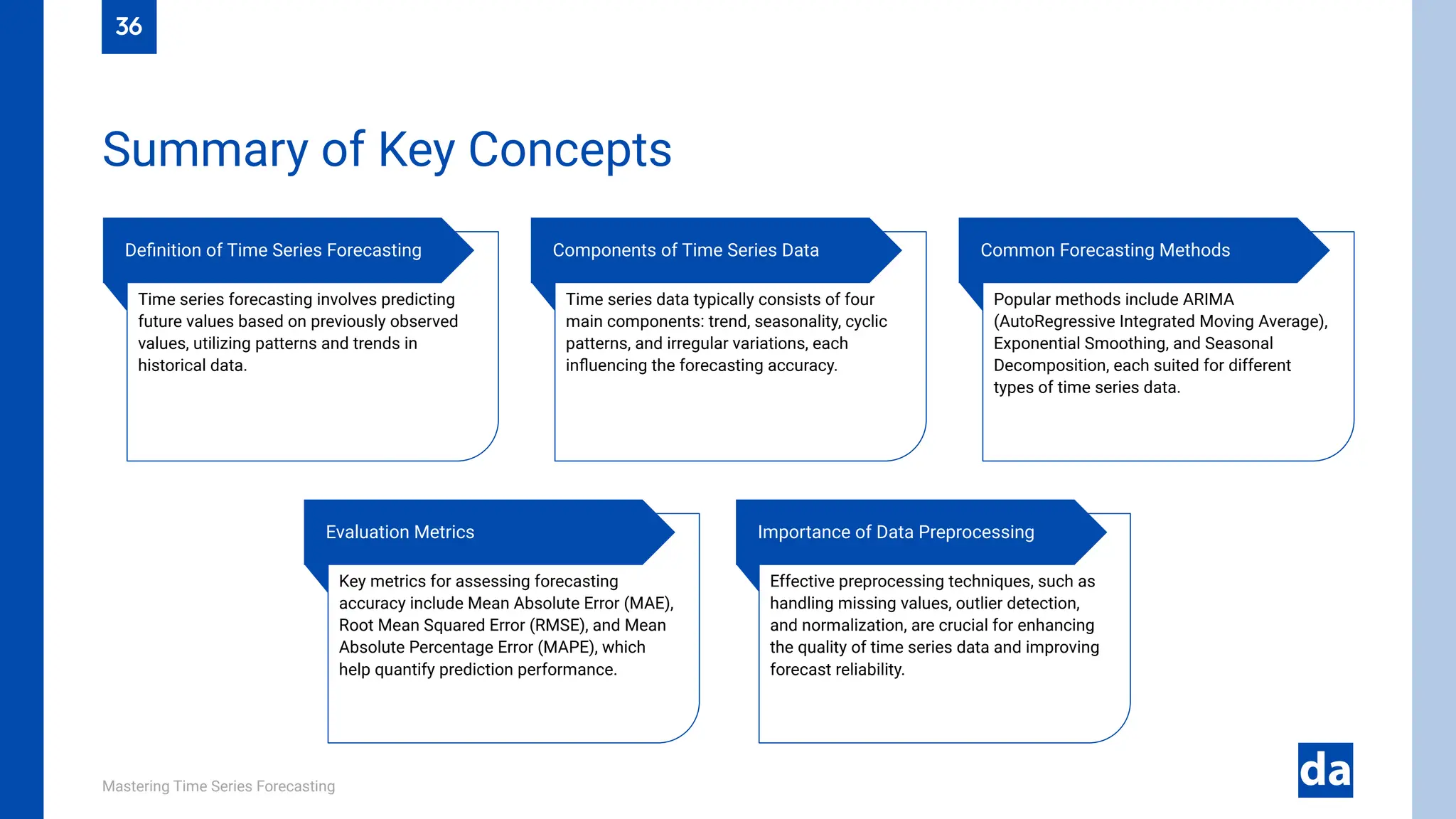
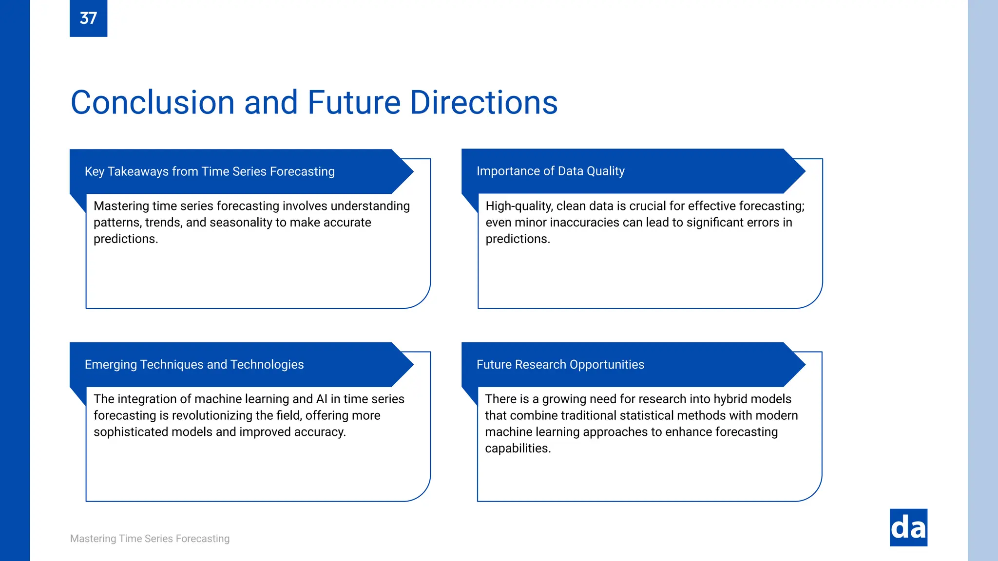

The document serves as a comprehensive guide to time series forecasting, covering techniques, applications, and future trends. It details the importance of time series analysis, types of data, various forecasting methods including ARIMA, SARIMA, and machine learning approaches like LSTM, and evaluation metrics for accuracy. Additionally, it discusses real-world applications in sectors such as finance, healthcare, and retail, as well as challenges and future trends in the field.


![[DSC Europe 25] Jim Sterne - Adopting Generative AI Capabilities Into the Ent...](https://cdn.slidesharecdn.com/ss_thumbnails/sxhpofuorcagxsaulkmt-3-251204082258-7e66bc48-thumbnail.jpg?width=640&height=640&fit=bounds)


![[DSC Europe 25] Dragan Vucic - Building the Learning Organization - How AI Tr...](https://cdn.slidesharecdn.com/ss_thumbnails/8brigo2sbu6qur6gxrra-7-251205085715-6ae07d24-thumbnail.jpg?width=640&height=640&fit=bounds)


![[DSC Europe 25] Petar Zivanov - AI meets documents From chatbots to AI-powere...](https://cdn.slidesharecdn.com/ss_thumbnails/xer2bb6nrdc8pdpev0pc-8-251204082258-7c2fa4a1-thumbnail.jpg?width=640&height=640&fit=bounds)
![[DSC Europe 25] Andy Cotgreave - Nothing is new in analytics.pptx](https://cdn.slidesharecdn.com/ss_thumbnails/mba4vzcurvoh5lfrd5zw-6-251205194645-341bbbbe-thumbnail.jpg?width=640&height=640&fit=bounds)

![[DSC Europe 25] Bogdan Daniel Maruneac - AI - It starts with you.pptx](https://cdn.slidesharecdn.com/ss_thumbnails/odov3snhrcqs9hx5ny2n-4-251205085715-f1daacfe-thumbnail.jpg?width=640&height=640&fit=bounds)


![[DSC Europe 25] Nikola Rajovic - Hardware Technologies Under the Hood: RISC-V...](https://cdn.slidesharecdn.com/ss_thumbnails/o2gptrmtoyqndgoshwgq-dsc2025-tenstorrent-rajovic-251205090438-814685f5-thumbnail.jpg?width=640&height=640&fit=bounds)

![[DSC Europe 25] Dragana Ilic - AI for Big Data in Astronomy.pptx](https://cdn.slidesharecdn.com/ss_thumbnails/8palya86qaatvjhva1ms-2-dragana-ilic-ai-ilic-251208151906-652b819c-thumbnail.jpg?width=640&height=640&fit=bounds)

![[DSC Europe 25] Goran Obradovic - The Rise of Sovereign AI: Building the Regi...](https://cdn.slidesharecdn.com/ss_thumbnails/7nw2xxixrxqdxvrb5wca-6-251205085714-ab09a2ac-thumbnail.jpg?width=640&height=640&fit=bounds)