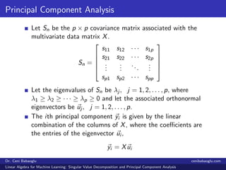
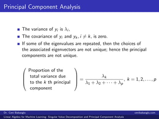
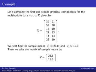
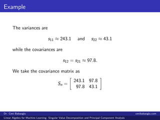
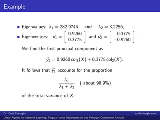
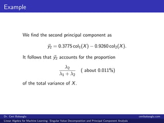
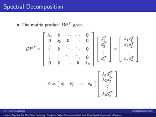
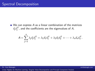
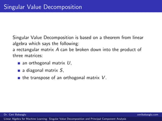
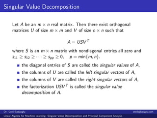
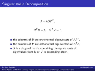
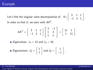
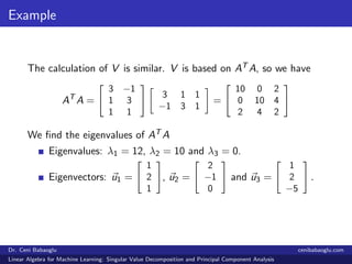
5. Linear Algebra for Machine Learning: Singular Value Decomposition and Principal Component Analysis

Seminar Series on
Linear Algebra for Machine Learning
Part 5: Singular Value Decomposition and
Principal Component Analysis
Dr. Ceni Babaoglu
Data Science Laboratory
Ryerson University
cenibabaoglu.com
Dr. Ceni Babaoglu cenibabaoglu.com
Linear Algebra for Machine Learning: Singular Value Decomposition and Principal Component Analysis

Overview
1 Spectral Decomposition
2 Singular Value Decomposition
3 Principal Component Analysis
4 References

Spectral Decomposition
An n × n symmetric matrix A can be expressed as the matrix
product
A = PDPT
where D is a diagonal matrix and P is an orthogonal matrix.
The diagonal entries of D are the eigenvalues of A,
λ1, λ2, · · · , λn, and the columns of P are associated
orthonormal eigenvectors x1, x2, · · · , xn.

The expression
A = PDPT
is called the spectral decomposition of A. We can write it as
A = x1 x2 · · · xn








λ1 0 · · · · · · 0
0 λ2 0 · · · 0
... 0
...
... 0
...
...
...
... 0
0 0 · · · 0 λn













xT
1
xT
2
...
xT
n






The matrix product DPT gives
DPT
=








λ1 0 · · · · · · 0
0 λ2 0 · · · 0
... 0
...
... 0
...
...
...
... 0
0 0 · · · 0 λn













xT
1
xT
2
...
xT
n





=





λ1xT
1
λ2xT
2
...
λnxT
n





A = x1 x2 · · · xn





λ1xT
1
λ2xT
2
...
λnxT
n






We can express A as a linear combination of the matrices
xj xT
j , and the coeﬃcients are the eigenvalues of A,
A =
n
j=1
λj xj xT
j = λ1x1xT
1 + λ2x2xT
2 + · · · + λnxnxT
n .

Singular Value Decomposition
Singular Value Decomposition is based on a theorem from linear
algebra which says the following:
a rectangular matrix A can be broken down into the product of
three matrices:
an orthogonal matrix U,
a diagonal matrix S,
the transpose of an orthogonal matrix V .

Let A be an m × n real matrix. Then there exist orthogonal
matrices U of size m × m and V of size n × n such that
A = USV T
where S is an m × n matrix with nondiagonal entries all zero and
s11 ≥ s12 ≥ · · · ≥ spp ≥ 0, p = min{m, n}.
the diagonal entries of S are called the singular values of A,
the columns of U are called the left singular vectors of A,
the columns of V are called the right singular vectors of A,
the factorization USV T is called the singular value
decomposition of A.

A = USV T
,
UT
U = I, V T
V = I,
the columns of U are orthonormal eigenvectors of AAT ,
the columns of V are orthonormal eigenvectors of AT A,
S is a diagonal matrix containing the square roots of
eigenvalues from U or V in descending order.

Example
Let’s ﬁnd the singular value decomposition of A=
3 1 1
−1 3 1
.
In order to ﬁnd U, we start with AAT .
AAT
=
3 1 1
−1 3 1


3 −1
1 3
1 1

 =
11 1
1 11
Eigenvalues: λ1 = 12 and λ2 = 10.
Eigenvectors: u1 =
1
1
and u2 =
1
−1
.

Example
Using Gram-Schmidt Process
v1 = u1 w1 =
v1
|v1|
=
1/
√
2
1/
√
2
v2 = u2 −
(u2, v1)
(v1, v1)
v1
v2 =
1
−1
− 0
1
1
=
1
−1
− [0, 0] =
1
−1
w2 =
v2
|v2|
=
1
√
2
,
−1
√
2
U =
1/
√
2 1/
√
2
1/
√
2 −1/
√
2

Example
The calculation of V is similar. V is based on AT A, so we have
AT
A =
3 −1
1 3
1 1
3 1 1
−1 3 1
=
10 0 2
0 10 4
2 4 2
We ﬁnd the eigenvalues of AT A
Eigenvalues: λ1 = 12, λ2 = 10 and λ3 = 0.
Eigenvectors: u1 =
1
2
1
, u2 =
2
−1
0
and u3 =
1
2
−5
.

Example
v1 = u1, w1 =
v1
|v1|
=
1
√
6
,
2
√
6
,
1
√
6
v2 = u2 −
(u2, v1)
(v1, v1)
v1 = [2, −1, 0]
w2 =
v2
|v2|
=
2
√
5
,
−1
√
5
, 0

Example
v3 = u3 −
(u3, v1)
(v1, v1)
v1 −
(u3, v2)
(v2, v2)
v2 =
−2
3
,
−4
3
,
10
3
w3 =
v3
|v3|
=
1
√
30
,
2
√
30
,
−5
√
30
V =



1√
6
2√
5
1√
30
2√
6
−1√
5
2√
30
1√
6
0 −5√
30


 , V T
=



1√
6
2√
6
1√
6
2√
5
−1√
5
0
1√
30
2√
30
−5√
30




Example
A = USV T
A =
1√
2
1√
2
1√
2
−1√
2
√
12 0 0
0
√
10 0


1√
6
2√
6
1√
6
2√
5
−1√
5
0
1√
30
2√
30
−5√
30

 =
3 1 1
−1 3 1

Let λ1, λ2, · · · , λn be the eigenvalues of A and x1, x2, · · · , xn be a
set of associated orthonormal eigenvectors.
Then the spectral decomposition of A is given by
A = λ1x1xT
1 + λ2x2xT
2 + · · · + λnxnxT
n .
If A is a real n × n matrix with real eigenvalues λ1, λ2, · · · , λn,
then an eigenvalue of largest magnitude is called a dominant
eigenvalue of A.

Let X be the multivariate data matrix
X =








x11 x12 · · · x1k · · · x1p
x21 x22 · · · x2k · · · x2p
...
...
...
...
xj1 xj2 · · · xjk · · · xjp
...
...
...
...
xn1 xn2 · · · xnk · · · xnp








.
The measure of association between the ith and kth variables in
the multivariate data matrix is given by the sample covariance
sik =
1
n
n
j=1
(xji − xi ) (xjk − xk) , i = 1, 2, . . . , p, k = 1, 2, . . . , p.

Let Sn be the p × p covariance matrix associated with the
multivariate data matrix X.
Sn =





s11 s12 · · · s1p
s21 s22 · · · s2p
...
...
...
...
sp1 sp2 · · · spp





Let the eigenvalues of Sn be λj , j = 1, 2, . . . , p, where
λ1 ≥ λ2 ≥ · · · ≥ λp ≥ 0 and let the associated orthonormal
eigenvectors be uj , j = 1, 2, . . . , p.
The ith principal component yi is given by the linear
combination of the columns of X, where the coeﬃcients are
the entries of the eigenvector ui ,
yi = Xui

The variance of yi is λi ,
The covariance of yi and yk, i = k, is zero.
If some of the eigenvalues are repeated, then the choices of
the associated eigenvectors are not unique; hence the principal
components are not unique.




Proportion of the
total variance due
to the k th principal
component



 =
λk
λ1 + λ2 + · · · + λp
, k = 1, 2, . . . , p

Example
Let’s compute the first and second principal components for the
multivariate data matrix X given by
X =








39 21
59 28
18 10
21 13
14 13
22 10








.
We first find the sample means x1 ≈ 28.8 and x2 ≈ 15.8.
Then we take the matrix of sample means as
x =
28.8
15.8

Example
The variances are
s11 ≈ 243.1 and s22 ≈ 43.1
while the covariances are
s12 = s21 ≈ 97.8.
We take the covariance matrix as
Sn =
243.1 97.8
97.8 43.1

Example
Eigenvalues: λ1 = 282.9744 and λ2 = 3.2256,
Eigenvectors: u1 =
0.9260
0.3775
and u2 =
0.3775
−0.9260
.
We ﬁnd the ﬁrst principal component as
y1 = 0.9260 col1(X) + 0.3775 col2(X).
It follows that y1 accounts for the proportion
λ1
λ1 + λ2
( about 98.9%)
of the total variance of X.

Example
We ﬁnd the second principal component as
y2 = 0.3775 col1(X) − 0.9260 col2(X).
It follows that y2 accounts for the proportion
λ2
λ1 + λ2
( about 0.011%)
of the total variance of X.

References
Linear Algebra With Applications, 7th Edition
by Steven J. Leon.
Elementary Linear Algebra with Applications, 9th Edition
by Bernard Kolman and David Hill.

5. Linear Algebra for Machine Learning: Singular Value Decomposition and Principal Component Analysis

More Related Content

What's hot

Similar to 5. Linear Algebra for Machine Learning: Singular Value Decomposition and Principal Component Analysis

Recently uploaded

5. Linear Algebra for Machine Learning: Singular Value Decomposition and Principal Component Analysis