detection therory

1. EC 622 Statistical Signal Processing
P. K. Bora
Department of Electronics & Communication Engineering
INDIAN INSTITUTE OF TECHNOLOGY GUWAHATI
1

2. EC 622 Statistical Signal Processing Syllabus
1. Review of random variables: distribution and density functions, moments, independent,
uncorrelated and orthogonal random variables; Vector-space representation of Random
variables, Schwarz Inequality Orthogonality principle in estimation, Central Limit
theorem, Random process, stationary process, autocorrelation and autocovariance
functions, Spectral representation of random signals, Wiener Khinchin theorem,
Properties of power spectral density, Gaussian Process and White noise process
2. Linear System with random input, Spectral factorization theorem and its importance,
innovation process and whitening filter
3. Random signal modelling: MA(q), AR(p) , ARMA(p,q) models
4. Parameter Estimation Theory: Principle of estimation and applications, Properties of
estimates, unbiased and consistent estimators, MVUE, CR bound, Efficient estimators;
Criteria of estimation: the methods of maximum likelihood and its properties ; Baysean
estimation: Mean Square error and MMSE, Mean Absolute error, Hit and Miss cost
function and MAP estimation
5. Estimation of signal in presence of White Gaussian Noise (WGN)
Linear Minimum Mean-Square Error (LMMSE) Filtering: Wiener Hoff Equation
FIR Wiener filter, Causal IIR Wiener filter, Noncausal IIR Wiener filter
Linear Prediction of Signals, Forward and Backward Predictions, Levinson Durbin
Algorithm, Lattice filter realization of prediction error filters
6. Adaptive Filtering: Principle and Application, Steepest Descent Algorithm
Convergence characteristics; LMS algorithm, convergence, excess mean square error
Leaky LMS algorithm; Application of Adaptive filters ;RLS algorithm, derivation,
Matrix inversion Lemma, Intialization, tracking of nonstationarity
7. Kalman filtering: Principle and application, Scalar Kalman filter, Vector Kalman filter
8. Spectral analysis: Estimated autocorrelation function, periodogram, Averaging the
periodogram (Bartlett Method), Welch modification, Blackman and Tukey method of
smoothing periodogram, Parametric method, AR(p) spectral estimation and detection of
Harmonic signals, MUSIC algorithm.
2

3. Acknowledgement
I take this opportunity to thank Prof. A. Mahanta who inspired me to take the course
Statistical Signal Processing. I am also thankful to my other faculty colleagues of the
ECE department for their constant support. I acknowledge the help of my students,
particularly Mr. Diganta Gogoi and Mr. Gaurav Gupta for their help in preparation of the
handouts. My appreciation goes to Mr. Sanjib Das who painstakingly edited the final
manuscript and prepared the power-point presentations for the lectures. I acknowledge
the help of Mr. L.N. Sharma and Mr. Nabajyoti Dutta for word-processing a part of the
manuscript. Finally I acknowledge QIP, IIT Guwhati for the financial support for this
work.
3

4. SECTION – I
REVIEW OF
RANDOM VARIABLES & RANDOM PROCESS
4

5. Table of Contents
CHAPTER - 1: REVIEW OF RANDOM VARIABLES ..............................................9
1.1 Introduction..............................................................................................................9
1.2 Discrete and Continuous Random Variables ......................................................10
1.3 Probability Distribution Function........................................................................10
1.4 Probability Density Function ...............................................................................11
1.5 Joint random variable ...........................................................................................12
1.6 Marginal density functions....................................................................................12
1.7 Conditional density function.................................................................................13
1.8 Baye’s Rule for mixed random variables.............................................................14
1.9 Independent Random Variable ............................................................................15
1.10 Moments of Random Variables..........................................................................16
1.11 Uncorrelated random variables..........................................................................17
1.12 Linear prediction of Y from X ..........................................................................17
1.13 Vector space Interpretation of Random Variables...........................................18
1.14 Linear Independence ...........................................................................................18
1.15 Statistical Independence......................................................................................18
1.16 Inner Product .......................................................................................................18
1.17 Schwary Inequality..............................................................................................19
1.18 Orthogonal Random Variables...........................................................................19
1.19 Orthogonality Principle.......................................................................................20
1.20 Chebysev Inequality.............................................................................................21
1.21 Markov Inequality ...............................................................................................21
1.22 Convergence of a sequence of random variables ..............................................22
1.23 Almost sure (a.s.) convergence or convergence with probability 1.................22
1.24 Convergence in mean square sense ....................................................................23
1.25 Convergence in probability.................................................................................23
1.26 Convergence in distribution................................................................................24
1.27 Central Limit Theorem .......................................................................................24
1.28 Jointly Gaussian Random variables...................................................................25
CHAPTER - 2 : REVIEW OF RANDOM PROCESS.................................................26
2.1 Introduction............................................................................................................26
2.2 How to describe a random process?.....................................................................27
2.3 Stationary Random Process..................................................................................28
2.4 Spectral Representation of a Random Process ...................................................30
2.5 Cross-correlation & Cross power Spectral Density............................................31
2.6 White noise process................................................................................................32
2.7 White Noise Sequence............................................................................................33
2.8 Linear Shift Invariant System with Random Inputs..........................................33
2.9 Spectral factorization theorem .............................................................................35
2.10 Wold’s Decomposition.........................................................................................37
CHAPTER - 3: RANDOM SIGNAL MODELLING ...................................................38
3.1 Introduction............................................................................................................38
3.2 White Noise Sequence............................................................................................38
3.3 Moving Average model )(qMA model ..................................................................38
3.4 Autoregressive Model............................................................................................40
3.5 ARMA(p,q) – Autoregressive Moving Average Model ......................................42
3.6 General ),( qpARMA Model building Steps .........................................................43
3.7 Other model: To model nonstatinary random processes...................................43
5

6. CHAPTER – 4: ESTIMATION THEORY ...................................................................45
4.1 Introduction............................................................................................................45
4.2 Properties of the Estimator...................................................................................46
4.3 Unbiased estimator ................................................................................................46
4.4 Variance of the estimator......................................................................................47
4.5 Mean square error of the estimator .....................................................................48
4.6 Consistent Estimators............................................................................................48
4.7 Sufficient Statistic ..................................................................................................49
4.8 Cramer Rao theorem.............................................................................................50
4.9 Statement of the Cramer Rao theorem................................................................51
4.10 Criteria for Estimation........................................................................................54
4.11 Maximum Likelihood Estimator (MLE) ...........................................................54
4.12 Bayescan Estimators............................................................................................56
4.13 Bayesean Risk function or average cost............................................................57
4.14 Relation between MAP
ˆθ and MLE
ˆθ ........................................................................62
CHAPTER – 5: WIENER FILTER...............................................................................65
5.1 Estimation of signal in presence of white Gaussian noise (WGN).....................65
5.2 Linear Minimum Mean Square Error Estimator...............................................67
5.3 Wiener-Hopf Equations ........................................................................................68
5.4 FIR Wiener Filter ..................................................................................................69
5.5 Minimum Mean Square Error - FIR Wiener Filter...........................................70
5.6 IIR Wiener Filter (Causal)....................................................................................74
5.7 Mean Square Estimation Error – IIR Filter (Causal)........................................76
5.8 IIR Wiener filter (Noncausal)...............................................................................78
5.9 Mean Square Estimation Error – IIR Filter (Noncausal)..................................79
CHAPTER – 6: LINEAR PREDICTION OF SIGNAL...............................................82
6.1 Introduction............................................................................................................82
6.2 Areas of application...............................................................................................82
6.3 Mean Square Prediction Error (MSPE)..............................................................83
6.4 Forward Prediction Problem................................................................................84
6.5 Backward Prediction Problem..............................................................................84
6.6 Forward Prediction................................................................................................84
6.7 Levinson Durbin Algorithm..................................................................................86
6.8 Steps of the Levinson- Durbin algorithm.............................................................88
6.9 Lattice filer realization of Linear prediction error filters..................................89
6.10 Advantage of Lattice Structure ..........................................................................90
CHAPTER – 7: ADAPTIVE FILTERS.........................................................................92
7.1 Introduction............................................................................................................92
7.2 Method of Steepest Descent...................................................................................93
7.3 Convergence of the steepest descent method.......................................................95
7.4 Rate of Convergence..............................................................................................96
7.5 LMS algorithm (Least – Mean –Square) algorithm...........................................96
7.6 Convergence of the LMS algorithm.....................................................................99
7.7 Excess mean square error ...................................................................................100
7.8 Drawback of the LMS Algorithm.......................................................................101
7.9 Leaky LMS Algorithm ........................................................................................103
7.10 Normalized LMS Algorithm.............................................................................103
7.11 Discussion - LMS ...............................................................................................104
7.12 Recursive Least Squares (RLS) Adaptive Filter.............................................105
6

7. 7.13 Recursive representation of ][ˆ nYYR ...............................................................106
7.14 Matrix Inversion Lemma ..................................................................................106
7.15 RLS algorithm Steps..........................................................................................107
7.16 Discussion – RLS................................................................................................108
7.16.1 Relation with Wiener filter ............................................................................108
7.16.2. Dependence condition on the initial values..................................................109
7.16.3. Convergence in stationary condition............................................................109
7.16.4. Tracking non-staionarity...............................................................................110
7.16.5. Computational Complexity...........................................................................110
CHAPTER – 8: KALMAN FILTER ...........................................................................111
8.1 Introduction..........................................................................................................111
8.2 Signal Model.........................................................................................................111
8.3 Estimation of the filter-parameters....................................................................115
8.4 The Scalar Kalman filter algorithm...................................................................116
8.5 Vector Kalman Filter...........................................................................................117
CHAPTER – 9 : SPECTRAL ESTIMATION TECHNIQUES FOR STATIONARY
SIGNALS........................................................................................................................119
9.1 Introduction..........................................................................................................119
9.2 Sample Autocorrelation Functions.....................................................................120
9.3 Periodogram (Schuster, 1898).............................................................................121
9.4 Chi square distribution........................................................................................124
9.5 Modified Periodograms.......................................................................................126
9.5.1 Averaged Periodogram: The Bartlett Method..............................................126
9.5.2 Variance of the averaged periodogram...........................................................128
9.6 Smoothing the periodogram : The Blackman and Tukey Method .................129
9.7 Parametric Method..............................................................................................130
9.8 AR spectral estimation ........................................................................................131
9.9 The Autocorrelation method...............................................................................132
9.10 The Covariance method ....................................................................................132
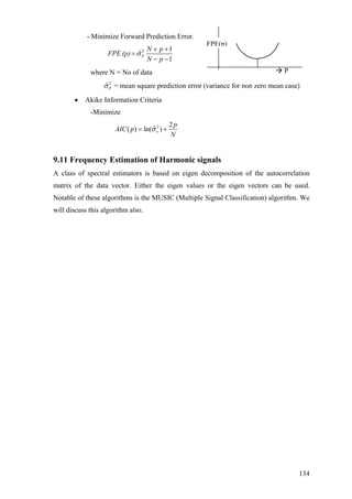
9.11 Frequency Estimation of Harmonic signals ....................................................134
10. Text and Reference..................................................................................................135
7

8. SECTION – I
REVIEW OF
RANDOM VARIABLES & RANDOM PROCESS
8

9. CHAPTER - 1: REVIEW OF RANDOM VARIABLES
1.1 Introduction
• Mathematically a random variable is neither random nor a variable
• It is a mapping from sample space into the real-line ( “real-valued” random
variable) or the complex plane ( “complex-valued ” random variable) .
Suppose we have a probability space },,{ PS ℑ .
Let be a function mapping the sample space into the real line such thatℜ→SX : S
For each there exists a unique .,Ss ∈ )( ℜ∈sX Then X is called a random variable.
Thus a random variable associates the points in the sample space with real numbers.
( )X s
ℜ
S
s •
Figure Random Variable
Notations:
• Random variables are represented by
upper-case letters.
• Values of a random variable are
denoted by lower case letters
• Y y= means that is the value of a
random variable
y
.X
Example 1: Consider the example of tossing a fair coin twice. The sample space is S=
{HH, HT, TH, TT} and all four outcomes are equally likely. Then we can define a
random variable X as follows
Sample Point Value of the random
Variable X x=
{ }P X x=
HH 0 1
4
HT 1 1
4
TH 2 1
4
TT 3 1
4
9

10. Example 2: Consider the sample space associated with the single toss of a fair die. The
sample space is given by . If we define the random variable{1,2,3,4,5,6}S = X that
associates a real number equal to the number in the face of the die, then {1,2,3,4,5,6}X =
1.2 Discrete and Continuous Random Variables
• A random variable X is called discrete if there exists a countable sequence of
distinct real number such thati
x ( ) 1m i
i
P x =∑ . is called the
probability mass function. The random variable defined in Example 1 is a
discrete random variable.
( )m iP x
• A continuous random variable X can take any value from a continuous
interval
• A random variable may also de mixed type. In this case the RV takes
continuous values, but at each finite number of points there is a finite
probability.
1.3 Probability Distribution Function
We can define an event S}s,)(/{}{ ∈≤=≤ xsXsxX
The probability
}{)( xXPxFX ≤= is called the probability distribution function.
Given ( ),XF x we can determine the probability of any event involving values of the
random variable .X
• is a non-decreasing function of)(xFX .X
• is right continuous)(xFX
=> approaches to its value from right.)(xFX
• 0)( =−∞XF
• 1)( =∞XF
• 1 1{ } ( )X XP x X x F x F x< ≤ = − ( )
10

11. Example 3: Consider the random variable defined in Example 1. The distribution
function ( )XF x is as given below:
Value of the random Variable X x= ( )XF x
0x < 0
0 1x≤ < 1
4
1 2x≤ < 1
2
2 3x≤ < 3
4
3x ≥ 1
( )XF x
X x=
1.4 Probability Density Function
If is differentiable)(xFX )()( xF
dx
d
xf XX = is called the probability density function and
has the following properties.
• is a non- negative function)(xf X
• ∫
∞
∞−
= 1)( dxxfX
• ∫−
=≤<
2
1
)()( 21
x
x
X dxxfxXxP
Remark: Using the Dirac delta function we can define the density function for a discrete
random variables.
11

12. 1.5 Joint random variable
X and are two random variables defined on the same sample space .
is called the joint distribution function and denoted by
Y S
},{ yYxXP ≤≤ ).,(, yxF YX
Given ,),,(, y, -x-yxF YX ∞<<∞∞<<∞ we have a complete description of the
random variables X and .Y
• ),(),0()0,(),(}0,0{ ,,,, yxFyFxFyxFyYxXP YXYXYXYX +−−=≤<≤<
• ).,()( +∞= xFxF XYX
To prove this
( ) ( ) ),(,)(
)()()(
+∞=∞≤≤=≤=∴
+∞≤∩≤=≤
xFYxXPxXPxF
YxXxX
XYX
( ) ( ) ),(,)( +∞=∞≤≤=≤= xFYxXPxXPxF XYX
Similarly ).,()( yFyF XYY ∞=
• Given ,),,(, y, -x-yxF YX ∞<<∞∞<<∞ each of is
called a marginal distribution function.
)(and)( yFxF YX
We can define joint probability density function , ( , ) of the random variables andX Yf x y X Y
by
2
, ( , ) ( , )X Y X Y,f x y F x y
x y
∂
=
∂ ∂
, provided it exists
• is always a positive quantity.),(, yxf YX
• ∫ ∫∞− ∞−
=
x
YX
y
YX dxdyyxfyxF ),(),( ,,
1.6 Marginal density functions
,
,
,
( ) ( )
( , )
( ( , ) )
( , )
an d ( ) ( , )
d
X Xd x
d
Xd x
x
d
X Yd x
X Y
Y X Y
f x F x
F x
f x y d y d x
f x y d y
f y f x y d x
∞
− ∞ − ∞
∞
− ∞
∞
− ∞
=
= ∞
= ∫ ∫
= ∫
= ∫
12

13. 1.7 Conditional density function
)/()/( // xyfxXyf XYXY == is called conditional density of Y given .X
Let us define the conditional distribution function.
We cannot define the conditional distribution function for the continuous random
variables andX Y by the relation
/
( / ) ( / )
( ,
=
( )
Y X
)
F y x P Y y X x
P Y y X x
P X x
= ≤ =
≤ =
=
as both the numerator and the denominator are zero for the above expression.
The conditional distribution function is defined in the limiting sense as follows:
0
/
0
,
0
,
( / ) ( / )
( ,
=l
( )
( , )
=l
( )
( , )
=
( )
x
Y X
x
y
X Y
x
X
y
X Y
X
)
F y x lim P Y y x X x x
P Y y x X x x
im
P x X x x
f x u xdu
im
f x x
f x u du
f x
∆ →
∆ →
∞
∆ →
∞
= ≤ < ≤
≤ < ≤ + ∆
< ≤ + ∆
∆∫
∆
∫
+ ∆
The conditional density is defined in the limiting sense as follows
(1)/))/()/((lim
/))/()/((lim)/(
//0,0
//0/
yxxXxyFxxXxyyF
yxXyFxXyyFxXyf
XYXYxy
XYXYyXY
∆∆+≤<−∆+≤<∆+=
∆=−=∆+==
→∆→∆
→∆
Because )(lim)( 0 xxXxxX x ∆+≤<== →∆
The right hand side in equation (1) is
0, 0 / /
0, 0
0, 0
lim ( ( / ) ( / ))/
lim ( ( / ))/
lim ( ( , ))/ ( )
y x Y X Y X
y x
y x
F y y x X x x F y x X x x y
P y Y y y x X x x y
P y Y y y x X x x P x X x x y
∆ → ∆ →
∆ → ∆ →
∆ → ∆ →
+ ∆ < < + ∆ − < < + ∆ ∆
= < ≤ + ∆ < ≤ + ∆ ∆
= < ≤ + ∆ < ≤ + ∆ < ≤
0, 0 ,
,
lim ( , ) / ( )
( , )/ ( )
y x X Y X
X Y X
f x y x y f x x y
f x y f x
∆ → ∆ →= ∆ ∆ ∆ ∆
=
+ ∆ ∆
,/ ( / ) ( , )/ ( )X Y XY Xf x y f x y f x∴ = (2)
Similarly, we have
,/ ( / ) ( , )/ ( )X Y YX Yf x y f x y f y∴ = (3)
13

14. From (2) and (3) we get Baye’s rule
,
/
/
,
,
/
/
( , )
( / )
( )
( ) ( / )
( )
( , )
=
( , )
( / ) ( )
=
( ) ( / )
X Y
X Y
Y
X Y X
Y
X Y
X Y
XY X
X Y X
f x y
f x y
f y
f x f y x
f y
f x y
f x y dx
f y x f x
f u f y x du
∞
−∞
∞
−∞
∴ =
=
∫
∫
(4)
Given the joint density function we can find out the conditional density function.
Example 4:
For random variables X and Y, the joint probability density function is given by
,
1
( , ) 1, 1
4
0 otherwise
X Y
xy
f x y x y
+
= ≤
=
≤
Find the marginal density /( ), ( ) and ( / ).X Y Y Xf x f y f y x Are independent?andX Y
1
1
1 1
( )
4 2
Similarly
1
( ) -1 1
2
X
Y
xy
f x dy
f y y
−
+
= =
= ≤ ≤
∫
and
,
/
( , ) 1
( / ) , 1, 1
( ) 4
= 0 otherwise
X Y
Y X
X
f x y xy
f y x x y
f x
+
= = ≤ ≤
and are not independentX Y∴
1.8 Baye’s Rule for mixed random variables
Let X be a discrete random variable with probability mass function and Y be a
continuous random variable. In practical problem we may have to estimate
( )XP x
X from
observed Then.Y
14

15. / 0 /
,
0
/
0
/
/
( / ) lim ( / )
( , )
= lim
( )
( ) ( / )
= lim
( )
( ) ( / )
=
( )
( ) (
= =
X Y y X Y
X Y
y
Y
X Y X
y
Y
X Y X
Y
X Y X
P x y P x y Y y y
P x y Y y y
P y Y y y
P x f y x y
f y y
P x f y x
f y
P x f
∆ →
∆ →
∆ →
= < ≤
< ≤ + ∆
< ≤ + ∆
∆
∆
+ ∆ ∞
/
/ )
( ) ( / )X Y X
x
y x
P x f y x∑
Example 5:
V
X
+ Y
X is a binary random variable with
1
1 with probability
2
1
1 with probability
2
X
⎧
⎪⎪
= ⎨
⎪−
⎪⎩
V is the Gaussian noise with mean
2
0 and variance .σ
Then
2 2
2 2 2 2
/
/
/
( 1) / 2
( 1) / 2 ( 1) / 2
( ) ( / )
( 1/ )
( ) ( / )
(
X Y X
X Y
X Y X
x
y
y y
P x f y x
P x y
P x f y x
e
e e
σ
σ σ
− −
− − − +
= =
∑
=
+
1.9 Independent Random Variable
Let X and Y be two random variables characterised by the joint density function
},{),(, yYxXPyxF YX ≤≤=
and ),(),( ,,
2
yxFyxf YXyxYX ∂∂
∂
=
Then X and Y are independent if / ( / ) ( )X Y Xf x y f x x= ∀ ∈ℜ
and equivalently
)()(),(, yfxfyxf YXYX = , where and are called the marginal
density functions.
)(xfX )(yfY
15

16. 1.10 Moments of Random Variables
• Expectation provides a description of the random variable in terms of a few
parameters instead of specifying the entire distribution function or the density
function
• It is far easier to estimate the expectation of a R.V. from data than to estimate its
distribution
First Moment or mean
The mean Xµ of a random variable X is defined by
( ) for a discrete random variable
( ) for a continuous random variable
X i i
X
EX x P x X
xf x dx X
µ
∞
−∞
= = ∑
= ∫
For any piecewise continuous function ( )y g x= , the expectation of the R.V.
is given by( )Y g X= ( ) ( ) ( )xEY Eg X g x f x dx
−∞
−∞
= = ∫
Second moment
2 2
( )XEX x f x
∞
−∞
= ∫ dx
X X
Variance
2 2
( ) ( )Xx f xσ µ
∞
−∞
= −∫ dx
• Variance is a central moment and measure of dispersion of the random variable
about the mean.
• xσ is called the standard deviation.
•
For two random variables X and Y the joint expectation is defined as
, ,( ) ( , )X Y X YE XY xyf x y dxdyµ
∞ ∞
−∞ −∞
= = ∫ ∫
The correlation between random variables X and Y measured by the covariance, is
given by
,
( , ) ( )( )
( - - )
( ) -
XY X Y
Y X X Y
X Y
Cov X Y E X Y
E XY X Y
E XY
σ µ µ
µ µ µ µ
µ µ
= = − −
= +
=
The ratio 2 2
( )( )
( ) ( )
X Y XY
X YX Y
E X Y
E X E Y
µ µ σ
ρ
σ σµ µ
− −
= =
− −
is called the correlation coefficient. The correlation coefficient measures how much two
random variables are similar.
16

17. 1.11 Uncorrelated random variables
Random variables X and Y are uncorrelated if covariance
0),( =YXCov
Two random variables may be dependent, but still they may be uncorrelated. If there
exists correlation between two random variables, one may be represented as a linear
regression of the others. We will discuss this point in the next section.
1.12 Linear prediction of Y from X
baXY +=ˆ Regression
Prediction error ˆY Y−
Mean square prediction error
2 2ˆ( ) ( )E Y Y E Y aX b− = − −
For minimising the error will give optimal values of Corresponding to the
optimal solutions for we have
.and ba
,and ba
2
2
( )
( )
E Y aX b
a
E Y aX b
b
∂ − − =
∂
∂ − − =
∂
0
0
Solving for ,ba and ,2
1ˆ (Y X Y
X
Y x )Xµ σ µ
σ
− = −
so that )(ˆ
, X
x
y
YXY xY µ
σ
σ
ρµ −=− , where
YX
XY
YX
σσ
σ
ρ =, is the correlation coefficient.
If 0, =YXρ then are uncorrelated.YX and
.predictionbesttheisˆ
0ˆ
Y
Y
Y
Y
µ
µ
==>
=−=>
Note that independence => Uncorrelatedness. But uncorrelated generally does not imply
independence (except for jointly Gaussian random variables).
Example 6:
(1,-1).betweenddistributeuniformlyisand2
(x)fXY X=
are dependent, but they are uncorrelated.YX and
Because
0)EX(
0
))((),(
3
==
===
−−==
∵EXEY
EXEXY
YXEYXCov YXX µµσ
In fact for any zero- mean symmetric distribution of X, are uncorrelated.2
and XX
17

18. 1.13 Vector space Interpretation of Random Variables
The set of all random variables defined on a sample space form a vector space with
respect to addition and scalar multiplication. This is very easy to verify.
1.14 Linear Independence
Consider the sequence of random variables .,...., 21 NXXX
If 0....2211 =+++ NN XcXcXc implies that
,0....21 ==== Nccc then are linearly independent..,...., 21 NXXX
1.15 Statistical Independence
NXXX ,...., 21 are statistically independent if
1 2 1 2, ,.... 1 2 1 2( , ,.... ) ( ) ( ).... ( )N NX X X N X X X Nf x x x f x f x f x=
Statistical independence in the case of zero mean random variables also implies linear
independence
1.16 Inner Product
If and are real vectors in a vector space V defined over the field , the inner productx y
>< yx, is a scalar such that
, , andx y z V a∀ ∈ ∈
2
1.
2. 0
3.
4.
x, y y,x
x,x x
x y,z x,z y,z
ax, y a x, y
< > = < >
< > = ≥
< + > = < > + <
< > = < >
>
YIn the case of RVs, inner product between is defined asandX
, , )X Y< X,Y >= EXY = xy f (x y dy dx.
∞ ∞
−∞ −∞
∫ ∫
Magnitude / Norm of a vector
>=< xxx ,
2
So, for R.V.
2 2 2
)XX EX = x f (x dx
∞
−∞
= ∫
• The set of RVs along with the inner product defined through the joint expectation
operation and the corresponding norm defines a Hilbert Space.
18

19. 1.17 Schwary Inequality
For any two vectors andx y belonging to a Hilbert space V
yx|x, y| ≤><
For RV andX Y
222
)( EYEXXYE ≤
Proof:
Consider the random variable YaXZ +=
.
02
0)(
222
2
≥⇒
≥+
aEXY++ EYEXa
YaXE
Non-negatively of the left-hand side => its minimum also must be nonnegative.
For the minimum value,
2
2
0
EX
EXY
a
da
dEZ
−==>=
so the corresponding minimum is 2
2
2
2
2
2
EX
XYE
EY
EX
XYE
−+
Minimum is nonnegative =>
222
2
2
2
0
EYEXXYE
EX
XYE
EY
<=>
≥−
2 2
( )( )( , )
( , )
( ) (
X Y
Xx X X Y
E X YCov X Y
X Y
E X E Y )
µ µ
ρ
σ σ µ µ
− −
= =
− −
From schwarz inequality
1),( ≤YXρ
1.18 Orthogonal Random Variables
Recall the definition of orthogonality. Two vectors are called orthogonal ifyx and
x, y 0=><
Similarly two random variables are called orthogonal ifYX and EXY 0=
If each of is zero-meanYX and
( , )Cov X Y EXY=
Therefore, if 0EXY = then Cov( ) 0XY = for this case.
For zero-mean random variables,
Orthogonality uncorrelatedness
19

20. 1.19 Orthogonality Principle
X is a random variable which is not observable. Y is another observable random variable
which is statistically dependent on X . Given a value of Y what is the best guess for X ?
(Estimation problem).
Let the best estimate be . Then is a minimum with respect
to .
)(ˆ YX 2
))(ˆ( YXXE −
)(ˆ YX
And the corresponding estimation principle is called minimum mean square error
principle. For finding the minimum, we have
2
ˆ
2
,ˆ
2
/ˆ
2
/ˆ
ˆ( ( )) 0
ˆ( ( )) ( , ) 0
ˆ( ( )) ( ) ( ) 0
ˆ( )( ( ( )) ( ) ) 0
X
X YX
Y X YX
Y X YX
E X X Y
x X y f x y dydx
x X y f y f x dydx
f y x X y f x dx dy
∂
∂
∞ ∞
∂
∂
−∞ −∞
∞ ∞
∂
∂
−∞ −∞
∞ ∞
∂
∂
−∞ −∞
− =
⇒ − =∫ ∫
⇒ −∫ ∫
⇒ −∫ ∫
=
=
Since in the above equation is always positive, therefore the
minimization is equivalent to
)(yfY
2
/ˆ
/
-
/ /
ˆ( ( )) ( ) 0
ˆOr 2 ( ( )) ( ) 0
ˆ ( ) ( ) ( )
ˆ ( ) ( / )
X YX
X Y
X Y X Y
x X y f x dx
x X y f x dx
X y f x dx xf x dx
X y E X Y
∞
∂
∂
−∞
∞
∞
∞ ∞
−∞ −∞
− =∫
− =∫
⇒ =∫ ∫
⇒ =
Thus, the minimum mean-square error estimation involves conditional expectation which
is difficult to obtain numerically.
Let us consider a simpler version of the problem. We assume that and the
estimation problem is to find the optimal value for Thus we have the linear
minimum mean-square error criterion which minimizes
ayyX =)(ˆ
.a
.)( 2
aYXE −
0
0)(
0)(
0)(
2
2
=⇒
=−⇒
=−⇒
=−
EeY
YaYXE
aYXE
aYXE
da
d
da
d
where e is the estimation error.
20

21. The above result shows that for the linear minimum mean-square error criterion,
estimation error is orthogonal to data. This result helps us in deriving optimal filters to
estimate a random signal buried in noise.
The mean and variance also give some quantitative information about the bounds of RVs.
Following inequalities are extremely useful in many practical problems.
1.20 Chebysev Inequality
Suppose X is a parameter of a manufactured item with known mean
2
and variance .X Xµ σ The quality control department rejects the item if the absolute
deviation of X from Xµ is greater than 2 X .σ What fraction of the manufacturing item
does the quality control department reject? Can you roughly guess it?
The standard deviation gives us an intuitive idea how the random variable is distributed
about the mean. This idea is more precisely expressed in the remarkable Chebysev
Inequality stated below. For a random variable X with mean 2
X Xµ σand variance
2
2{ } X
XP X σ
µ ε
ε
− ≥ ≤
Proof:
2
2 2
2
2
2
2
( ) ( )
( ) ( )
( )
{ }
{ }
X
X
X
x X X
X X
X
X
X
X
X
x f x dx
x f x dx
f x dx
P X
P X
µ ε
µ ε
σ
σ µ
µ
ε
ε µ ε
µ ε
ε
∞
−∞
− ≥
− ≥
= −∫
≥ −∫
≥ ∫
= − ≥
∴ − ≥ ≤
1.21 Markov Inequality
For a random variable X which take only nonnegative values
( )
{ }
E X
P X a
a
≥ ≤ where 0.a >
0
( ) ( )
( )
( )
{ }
X
X
a
X
a
E X xf x dx
xf x dx
af x dx
aP X a
∞
∞
∞
= ∫
≥ ∫
≥ ∫
= ≥
21

22. ( )
{ }
E X
P X a
a
∴ ≥ ≤
Result:
2
2 ( )
{( ) }
E X k
P X k a
a
−
− ≥ ≤
1.22 Convergence of a sequence of random variables
Let 1 2, ,..., nX X X be a sequence independent and identically distributed random
variables. Suppose we want to estimate the mean of the random variable on the basis of
the observed data by means of the relation
n
1
1
ˆ
N
X i
i
X
n
µ
=
= ∑
How closely does ˆXµ represent Xµ as is increased? How do we measure the
closeness between
n
ˆXµ and Xµ ?
Notice that ˆXµ is a random variable. What do we mean by the statement ˆXµ converges
to Xµ ?
Consider a deterministic sequence The sequence converges to a limit if
correspond to any
....,...., 21 nxxx x
0>ε we can find a positive integer such thatm for .nx x nε− < > m
Convergence of a random sequence cannot be defined as above.....,...., 21 nXXX
A sequence of random variables is said to converge everywhere to X if
( ) ( ) 0 for and .nX X n mξ ξ ξ− → > ∀
1.23 Almost sure (a.s.) convergence or convergence with probability 1
For the random sequence ....,...., 21 nXXX
}{ XX n → this is an event.
If
{ | ( ) ( )} 1 ,
{ ( ) ( ) for } 1 ,
n
n
P s X s X s as n
P s X s X s n m as mε
→ = → ∞
− < ≥ = → ∞
then the sequence is said to converge to X almost sure or with probability 1.
One important application is the Strong Law of Large Numbers:
If are iid random variables, then....,...., 21 nXXX
1
1
with probability 1as .
n
i X
i
X n
n
µ
=
→ →∑ ∞
22

23. 1.24 Convergence in mean square sense
If we say that the sequence converges to,0)( 2
∞→→− nasXXE n X in mean
square (M.S).
Example 7:
If are iid random variables, then....,...., 21 nXXX
1
1
in the mean square 1as .
N
i X
i
X n
n
µ
=
→ →∑ ∞
2
1
1
We have to show that lim ( ) 0
N
i X
n i
E X
n
µ
→∞ =
− =∑
Now,
2 2
1 1
n n
2
2 2
1 i=1 j=1,j i
2
2
1 1
( ) ( ( ( ))
1 1
( ) + ( )( )
+0 ( Because of independence)
N N
i X i X
i i
N
i X i X j X
i
X
E X E X
n n
E X E X X
n n
n
n
µ µ
µ µ
σ
= =
= ≠
− = −∑ ∑
= − − −∑ ∑ ∑
=
µ
2
2
1
1
lim ( ) 0
X
N
i X
n i
n
E X
n
σ
µ
→∞ =
=
∴ − =∑
1.25 Convergence in probability
}{ ε>− XXP n is a sequence of probability. is said to convergent tonX X in
probability if this sequence of probability is convergent that is
.0}{ ∞→→>− nasXXP n ε
If a sequence is convergent in mean, then it is convergent in probability also, because
2 2 2 2
{ } ( ) /n nP X X E X Xε− > ≤ − ε (Markov Inequality)
We have
22
/)(}{ εε XXEXXP nn −≤>−
If (mean square convergent) then,0)( 2
∞→→− nasXXE n
.0}{ ∞→→>− nasXXP n ε
23

24. Example 8:
Suppose { }nX be a sequence of random variables with
1
( 1} 1
and
1
( 1}
n
n
P X
n
P X
n
= = −
= − =
Clearly
1
{ 1 } { 1} 0
.
n nP X P X
n
as n
ε− > = = − = →
→ ∞
Therefore { } { 0}P
nX X⎯⎯→ =
1.26 Convergence in distribution
The sequence is said to converge to....,...., 21 nXXX X in distribution if
.)()( ∞→→ nasxFxF XXn
Here the two distribution functions eventually coincide.
1.27 Central Limit Theorem
Consider independent and identically distributed random variables .,...., 21 nXXX
Let nXXXY ...21 ++=
Then nXXXY µµµµ ...21
++=
And 2222
...21 nXXXY σσσσ +++=
The central limit theorem states that under very general conditions Y converges to
as The conditions are:),( 2
YYN σµ .∞→n
1. The random variables
1 2, ,..., nX X X are independent with same mean and
variance, but not identically distributed.
2. The random variables
1 2, ,..., nX X X are independent with different mean and
same variance and not identically distributed.
24

25. 1.28 Jointly Gaussian Random variables
Two random variables are called jointly Gaussian if their joint density function
is
YX and
2 2( ) ( )( ) ( )
1
2 2 22(1 ),
2
, ( , )
x x y y
X X Y Y
XY
X YX Y X Y
X Yf x y Ae
µ µ µ µ
σ σρ σ σ
ρ
− − − −
−
⎡ ⎤
− − +⎢ ⎥
⎢ ⎥⎣ ⎦
=
where 2
,12
1
YXyx
A
ρσπσ −
=
Properties:
(1) If X and Y are jointly Gaussian, then for any constants a and then the random
variable
,b
given by is Gaussian with mean,Z bYaXZ += YXZ ba µµµ += and variance
YXYXYXZ abba ,
22222
2 ρσσσσσ ++=
(2) If two jointly Gaussian RVs are uncorrelated, 0, =YXρ then they are statistically
independent.
)()(),(, yfxfyxf YXYX = in this case.
(3) If is a jointly Gaussian distribution, then the marginal densities),(, yxf YX
are also Gaussian.)(and)( yfxf YX
(4) If X and are joint by Gaussian random variables then the optimum nonlinear
estimator
Y
Xˆ of X that minimizes the mean square error is a linear
estimator
}]ˆ{[ 2
XXE −=ξ
aYX =ˆ
25

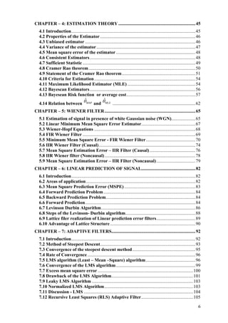
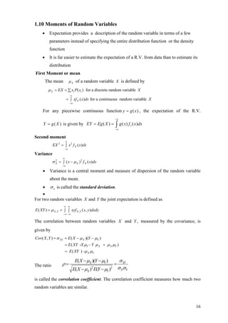
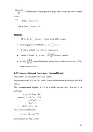
26. CHAPTER - 2 : REVIEW OF RANDOM PROCESS
2.1 Introduction
Recall that a random variable maps each sample point in the sample space to a point in
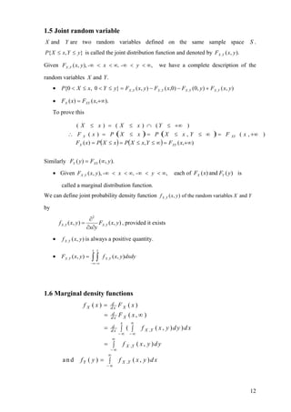
the real line. A random process maps each sample point to a waveform.
• A random process can be defined as an indexed family of random variables
{ ( ), }X t t T∈ whereT is an index set which may be discrete or continuous usually
denoting time.
• The random process is defined on a common probability space }.,,{ PS ℑ
• A random process is a function of the sample point ξ and index variable t and
may be written as ).,( ξtX
• For a fixed )),( 0tt = ,( 0 ξtX is a random variable.
• For a fixed ),( 0ξξ = ),( 0ξtX is a single realization of the random process and
is a deterministic function.
• When both andt ξ are varying we have the random process ).,( ξtX
The random process ),( ξtX is normally denoted by ).(tX
We can define a discrete random process [ ]X n on discrete points of time. Such a random
process is more important in practical implementations.
2( , )X t s3s
2s 1s
3( , )X t s
S
1( , )X t s
t
Figure Random Process
26

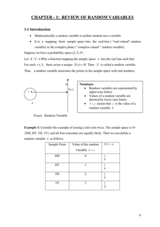
27. 2.2 How to describe a random process?
To describe we have to use joint density function of the random variables at
different .
)(tX
t
For any positive integer , represents jointly distributed
random variables. Thus a random process can be described by the joint distribution
function
n )(),.....(),( 21 ntXtXtX n
and),.....,,.....,().....,( 212121)().....(),( 21
TtNntttxxxFxxxF nnnntXtXtX n
∈∀∈∀=
Otherwise we can determine all the possible moments of the process.
)())(( ttXE xµ= = mean of the random process at .t
))()((),( 2121 tXtXEttRX = = autocorrelation function at 21,tt
))(),(),((),,( 321321 tXtXtXEtttRX = = Triple correlation function at etc.,,, 321 ttt
We can also define the auto-covariance function of given by),( 21 ttCX )(tX
)()(),(
))()())(()((),(
2121
221121
ttttR
ttXttXEttC
XXX
XXX
µµ
µµ
−=
−−=
Example 1:
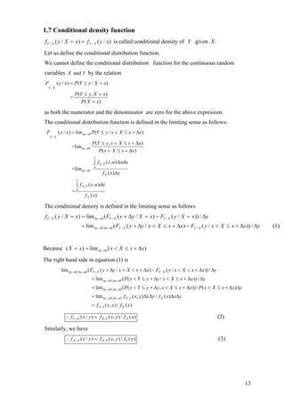
(a) Gaussian Random Process
For any positive integer represent jointly random
variables. These random variables define a random vector
The process is called Gaussian if the random vector
,n )(),.....(),( 21 ntXtXtX n
n
1 2[ ( ), ( ),..... ( )]'.nX t X t X t=X )(tX
1 2[ ( ), ( ),..... ( )]'nX t X t X t is jointly Gaussian with the joint density function given by
( )
' 1
1 2
1
2
( ), ( )... ( ) 1 2( , ,... )
2 det(
X
nX t X t X t n n
e
f x x x
π
−
−
=
XC X
XC )
Ewhere '( )( )= − −X X XC X µ X µ
and [ ]1 2( ) ( ), ( )...... ( ) '.nE E X E X E X= =Xµ X
(b) Bernouli Random Process
(c) A sinusoid with a random phase.
27

28. 2.3 Stationary Random Process
A random process is called strict-sense stationary if its probability structure is
invariant with time. In terms of the joint distribution function
)(tX
,and).....,().....,( 021)().....(),(21)().....(),( 0020121
TttNnxxxFxxxF nnttXttXttXntXtXtX nn
∈∀∈∀= +++
For ,1=n
)()( 01)(1)( 011
TtxFxF ttXtX ∈∀= +
Let us assume 10 tt −=
constant)0()0()(
)()(
1
1)0(1)( 1
===⇒
=
X
XtX
EXtEX
xFxF
µ
For ,2=n
),(.),( 21)(),(21)(),( 020121
xxFxxF ttXttXtXtX ++=
Put 20 tt −=
)(),(
),(),(
2121
21)0(),(21)(),( 2121
ttRttR
xxFxxF
XX
XttXtXtX
−=⇒
= −
A random process is called wide sense stationary process (WSS) if)(tX
1 2 1 2
( ) constant
( , ) ( ) is a function of time lag.
X
X X
t
R t t R t t
µ =
= −
For a Gaussian random process, WSS implies strict sense stationarity, because this
process is completely described by the mean and the autocorrelation functions.
The autocorrelation function )()()( tXtEXRX ττ += is a crucial quantity for a WSS
process.
• 2
0( )X ( )EX tR = is the mean-square value of the process.
• *
for real process (for a complex process ,( ) ( ) ( ) ( )XX X XX(t)R R R Rτ τ τ= −− τ=
• 0( ) ( )X XR Rτ < which follows from the Schwartz inequality
2 2
2
2 2
2 2
2 2
( ) { ( ) ( )}
( ), ( )
( ) ( )
( ) ( )
(0) (0)
0( ) ( )
X
X X
X X
R EX t X t
X t X t
X t X t
EX t EX t
R R
R R
τ τ
τ
τ
τ
τ
= +
= < + >
≤ +
= +
=
∴ <
28

29. • ( )XR τ is a positive semi-definite function in the sense that for any positive
integer and realn jj aa , ,
1 1
( , ) 0
n n
i j X i j
i j
a a R t t
= =
>∑ ∑
• If is periodic (in the mean square sense or any other sense like with
probability 1), then
)(tX
)(τXR is also periodic.
For a discrete random sequence, we can define the autocorrelation sequence similarly.
• If )(τXR drops quickly , then the signal samples are less correlated which in turn
means that the signal has lot of changes with respect to time. Such a signal has
high frequency components. If )(τXR drops slowly, the signal samples are highly
correlated and such a signal has less high frequency components.
• )(τXR is directly related to the frequency domain representation of WSS process.
The following figure illustrates the above concepts
Figure Frequency Interpretation of Random process: for slowly varying random process
Autocorrelation decays slowly
29

30. 2.4 Spectral Representation of a Random Process
How to have the frequency-domain representation of a random process?
• Wiener (1930) and Khinchin (1934) independently discovered the spectral
representation of a random process. Einstein (1914) also used the concept.
• Autocorrelation function and power spectral density forms a Fourier transform
pair
Lets define
otherwise0
Tt-TX(t)(t)XT
=
<<=
as will represent the random process)(, tXt T∞→ ).(tX
Define in mean square sense.dte(t)Xw)X jwt
T
T
TT
−
−
∫=(
τ−
2t
τ−
dτ
1t
2121
2*
21
)()(
2
1
2
|)(|
2
)()(
dtdteetXtEX
TT
X
E
T
XX
E tjtj
T
T
T
T
T
T
TTT ωωωωω +−
− −
∫ ∫==
= 1 2( )
1 2 1 2
1
( )
2
T T
j t t
X
T T
R t t e dt dt
T
ω− −
− −
−∫ ∫
=
2
2
1
( ) (2 | |)
2
T
j
X
T
R e T d
T
ωτ
τ τ−
−
−∫ τ
Substituting τ=− 21 tt so that τ−= 12 tt is a line, we get
τ
τ
τ
ωω ωτ
d
T
eR
T
XX
E j
T
T
x
TT
)
2
||
1()(
2
)()( 2
2
*
−= −
−
∫
If XR ( )τ is integrable then as ,∞→T
2
( )
lim ( )
2
T j
T X
E X
R e d
T
ωτω
τ τ
∞
−
→∞
−∞
= ∫
30

31. =
T
XE T
2
)(
2
ω
contribution to average power at freqω and is called the power spectral
density.
Thus
) ( )
) )
X
X X
S (
and R ( S (
j
x
j
R e d
e dw
ωτ
ωτ
ω τ τ
τ ω
∞
−
−∞
∞
−∞
=
=
∫
∫
Properties
• = average power of the process.2
XR (0) ( )XEX (t) S dwω
∞
−∞
= = ∫
• The average power in the band is1( , 2)w w
2
1
( )
w
X
w
S w dw∫
• )(RX τ is real and even )(ωXS⇒ is real, even.
• From the definition
2
( )
( ) lim
2
T
X T
E X
S w
T
ω
→∞= is always positive.
• ==
)(
)(
)( 2
tEX
S
wh x
X
ω
normalised power spectral density and has properties of PDF,
(always +ve and area=1).
2.5 Cross-correlation & Cross power Spectral Density
Consider two real random processes .and Y(t)X(t)
Joint stationarity of implies that the joint densities are invariant with shift
of time.
Y(t)X(t) and
The cross-correlation function for a jointly wss processes is
defined as
)X,YR (τ Y(t)X(t) and
))
)
)()(
)()()thatso
)()()
τ(R(τR
τ(R
τtYtXΕ
tXτtYΕ(τR
tYτtXΕ(τR
X,YYX
X,Y
YX
X,Y
−=∴
−=
+=
+=
+=
Cross power spectral density
, ,( ) ( ) jw
X Y X YS w R e dτ
τ τ
∞
−
−∞
= ∫
For real processes Y(t)X(t) and
31

32. *
, ,( ) ( )X Y Y XS w S w=
The Wiener-Khinchin theorem is also valid for discrete-time random processes.
If we define ][][][ nXmnE XmRX +=
Then corresponding PSD is given by
[ ]
[ ] 2
( )
or ( ) 1 1
j m
X x
m
j m
X x
m
S w R m e w
S f R m e f
ω
π
π π
∞
−
=−∞
∞
−
=−∞
= −∑
= −∑
≤ ≤
≤ ≤
1
[ ] ( )
2
j m
X XR m S w e
π
ω
ππ −
dw∫∴ =
For a discrete sequence the generalized PSD is defined in the domainz − as follows
[ ]( ) m
X x
m
S z R m z
∞
−
=−∞
= ∑
If we sample a stationary random process uniformly we get a stationary random sequence.
Sampling theorem is valid in terms of PSD.
Examples 2:
2 2
2
2
(1) ( ) 0
2
( ) -
(2) ( ) 0
1
( ) -
1 2 cos
a
X
X
m
X
X
R e a
a
S w w
a w
R m a a
a
S w w
a w a
τ
τ
π π
−
= >
= ∞ < <
+
= >
−
= ≤
− +
∞
≤
)
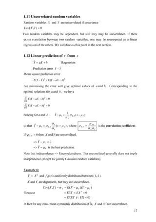
2.6 White noise process
S (x f
→ f
A white noise process is defined by)(tX
( )
2
X
N
S f f= −∞ < < ∞
The corresponding autocorrelation function is given by
( ) ( )
2
X
N
R τ δ τ= where )(τδ is the Dirac delta.
The average power of white noise
2
avg
N
P df
∞
−∞
= →∫ ∞
32

33. • Samples of a white noise process are uncorrelated.
• White noise is an mathematical abstraction, it cannot be realized since it has infinite
power
• If the system band-width(BW) is sufficiently narrower than the noise BW and noise
PSD is flat , we can model it as a white noise process. Thermal and shot noise are well
modelled as white Gaussian noise, since they have very flat psd over very wide band
(GHzs
• For a zero-mean white noise process, the correlation of the process at any lag 0≠τ is
zero.
• White noise plays a key role in random signal modelling.
• Similar role as that of the impulse function in the modeling of deterministic signals.
2.7 White Noise Sequence
For a white noise sequence ],[nx
( )
2
X
N
S w wπ π= − ≤ ≤
Therefore
( ) ( )
2
X
N
R m δ= m
where )(mδ is the unit impulse sequence.
White Noise WSS Random Signal
Linear
System
2.8 Linear Shi I va ia t yste ith Random Inputsft n r n S m w
Consider a discrete-time linear system with impulse response ].[nh
][][][
][][][
n* hnE xnE y
n* hnxny
=
=
For stationary input ][nx
0
[ ] [ ] [ ]
l
Y X X
k
E y n * h n h nµ µ µ
=
= = = ∑
2
N
2
N
2
N
( )XS ω
][nh
][nx
][ny
2
N
• • m• • →•
[ ]XR m
2
N
π ω→π−
33

34. where is the length of the impulse response sequencel
][*][*][
])[*][(*])[][(
][][][
mhmhmR
mnhmnxn* hnxE
mnynE ymR
X
Y
−=
−−=
−=
is a function of lag only.][mRY m
From above we get
w)SwΗ(wS XY (|(|= 2
))
)(wSXX
Example 3:
Suppose
X
( ) 1
0 otherwise
S ( )
2
c cH w w w
N
w w
= − ≤ ≤
=
= − ∞ ≤ ≤
w
∞
Then YS ( )
2
c c
N
w w w w= − ≤ ≤
and Y cR ( ) sinc(w )
2
N
τ τ=
2
)H(w
)(wSYY
)(τXR
τ
• Note that though the input is an uncorrelated process, the output is a correlated
process.
Consider the case of the discrete-time system with a random sequence as an input.][nx
][*][*][][ mhmhmRmR XY −=
Taking the we gettransform,−z
S )()()()( 1−
= zHzHzSz XY
Notice that if is causal, then is anti causal.)(zH )( 1−
zH
Similarly if is minimum-phase then is maximum-phase.)(zH )( 1−
zH
][nh
][nx ][ny
)(zH )( 1−
zH
][mRXX
][mRYY
][zSYY( )XXS z
34

35. Example 4:
If 1
1
( )
1
H z
zα −
=
−
and is a unity-variance white-noise sequence, then][nx
1
1
( ) ( ) ( )
1 1
1 21
YYS z H z H z
zz
1
α πα
−
−
=
⎛ ⎞⎛ ⎞
= ⎜ ⎟⎜ ⎟
−−⎝ ⎠⎝ ⎠
By partial fraction expansion and inverse −z transform, we get
||
2
1
1
][ m
Y amR
α−
=
2.9 Spectral factorization theorem
A stationary random signal that satisfies the Paley Wiener condition
can be considered as an output of a linea filter fed by a white noise
sequence.
][nX
| ln ( ) |XS w dw
π
π−
< ∞∫ r
If is an analytic function of ,)(wSX w
and , then| ln ( ) |XS w dw
π
π−
< ∞∫
2
( ) ( ) ( )X v c aS z H z H zσ=
where
)(zHc is the causal minimum phase transfer function
)(zHa is the anti-causal maximum phase transfer function
and 2
vσ a constant and interpreted as the variance of a white-noise sequence.
Innovation sequence
v n[ ] ][nX
Figure Innovation Filter
Minimum phase filter => the corresponding inverse filter exists.
)(zHc
Since is analytic in an annular region)(ln zSXX
1
zρ
ρ
< < ,
ln ( ) [ ] k
XX
k
S z c k z
∞
−
=−∞
= ∑
)
1
zHc
[ ]v n
(][nX
Figure whitening filter
35

36. where
1
[ ] ln ( )
2
iwn
XXc k S w e dwπ
π
π −= ∫ is the order cepstral coefficient.kth
For a real signal [ ] [ ]c k c k= −
and
1
[0] ln ( )
2
XXc Sπ
π
π −= ∫ w dw
1
1
1
[ ]
[ ] [ ]
[0]
[ ]
-1 2
( )
Let ( )
1 (1)z (2) ......
k
k
k k
k k
k
k
c k z
XX
c k z c k z
c
c k z
C
c c
S z e
e e e
H z e z
h h z
ρ
∞
−
=−∞
∞ −
− −
= =−∞
∞
−
=
∑
∑ ∑
∑
−
=
=
= >
= + + +
( [0] ( ) 1c z Ch Lim H z→∞= =∵
( )CH z and are both analyticln ( )CH z
=> is a minimum phase filter.( )CH z
Similarly let
1
1
( )
( )
1
( )
1
( )
k
k
a
k
k
c k z
c k z
C
H z e
e H z z
ρ
−
−
=−∞
∞
=
∑
∑
−
=
= = <
0)
2 1
Therefore,
( ) ( ) ( )XX V C CS z H z H zσ −
=
where 2 (c
V eσ =
Salient points
• can be factorized into a minimum-phase and a maximum-phase factors
i.e. and
)(zSXX
( )CH z 1
( )CH z−
.
• In general spectral factorization is difficult, however for a signal with rational
power spectrum, spectral factorization can be easily done.
• Since is a minimum phase filter, 1
( )CH z
exists (=> stable), therefore we can have a
filter
1
( )CH z
to filter the given signal to get the innovation sequence.
• and are related through an invertible transform; so they contain the
same information.
][nX [ ]v n
36

37. 2.10 Wold’s Decomposition
Any WSS signal can be decomposed as a sum of two mutually orthogonal
processes
][nX
• a regular process [ ]rX n and a predictable process [ ]pX n , [ ] [ ] [ ]r pX n X n X n= +
• [ ]rX n can be expressed as the output of linear filter using a white noise
sequence as input.
• [ ]pX n is a predictable process, that is, the process can be predicted from its own
past with zero prediction error.
37

38. CHAPTER - 3: RANDOM SIGNAL MODELLING
3.1 Introduction
The spectral factorization theorem enables us to model a regular random process as
an output of a linear filter with white noise as input. Different models are developed
using different forms of linear filters.
• These models are mathematically described by linear constant coefficient
difference equations.
• In statistics, random-process modeling using difference equations is known as
time series analysis.
3.2 White Noise Sequence
The simplest model is the white noise . We shall assume that is of 0-
mean and variance
[ ]v n [ ]v n
2
.Vσ
[ ]VR m
3.3 Moving Average model model)(qMA
[ ]v n ][ nX
The difference equation model is
[ ] [ ]
q
i
i o
X n b v n
=
i= −∑
2 2 2
0
0 0
and [ ] is an uncorrelated sequence means
e X
q
X i V
i
v n
b
µ µ
σ σ
=
= ⇒ =
= ∑
The autocorrelations are given by
• • • • m
FIR
filter
( )VS w 2
w
2
Vσ
π
38

39. 0 0
0 0
[ ] [ ] [ ]
[ ] [ ]
[ ]
X
q q
i j
i j
q q
i j V
i j
R m E X n X n - m
bb Ev n i v n m j
bb R m i j
= =
= =
=
= − − −∑ ∑
= − +∑ ∑
Noting that 2
[ ] [ ]V VR m σ δ= m , we get
2
[ ] when
0
V VR m
m-i j
i m j
σ=
+ =
⇒ = +
The maximum value for so thatqjm is+
2
0
[ ] 0
and
[ ] [ ]
q m
X j j m V
j
X X
R m b b m
R m R m
σ
−
+
=
= ≤∑
− =
q≤
Writing the above two relations together
2
0
[ ]
= 0 otherwise
q m
X j vj m
j
R m b b mσ
−
+
=
q= ≤∑
Notice that, [ ]XR m is related by a nonlinear relationship with model parameters. Thus
finding the model parameters is not simple.
The power spectral density is given by
2
2
( ) ( )
2
V
XS w B w
σ
π
= , where jqw
q
jw
ebebbwB −−
1 ++== ......)( ο
FIR system will give some zeros. So if the spectrum has some valleys then MA will fit
well.
3.3.1 Test for MA process
[ ]XR m becomes zero suddenly after some value of .m
[ ]XR m
m
Figure: Autocorrelation function of a MA process
39

40. Figure: Power spectrum of a MA process
Example 1: MA(1) process
1 0
0 1
2 2 2
1 0
1 0
[ ] [ 1] [ ]
Here the parameters b and are tobe determined.
We have
[1]
X
X
X n b v n b v n
b
b b
R b b
σ
= − +
= +
=
From above can be calculated using the variance and autocorrelation at lag 1 of
the signal.
0 andb 1b
3.4 Autoregressive Model
In time series analysis it is called AR(p) model.
The model is given by the difference equation
1
[ ] [ ] [ ]
p
i
i
X n a X n i v
=
= − +∑ n
The transfer function is given by)(wA
q m→
[ ]XR m( )XS w
ω→
][nXIIR
filter
[ ]v n
40

41. 1
1
( )
1
n
j i
i
i
A w
a e ω−
=
=
− ∑
with (all poles model) and10 =a
2
2
( )
2 | ( ) |
e
XS w
A
σ
π ω
=
If there are sharp peaks in the spectrum, the AR(p) model may be suitable.
The autocorrelation function [ ]XR m is given by
1
2
1
[ ] [ ] [ ]
[ ] [ ] [ ] [ ]
[ ] [ ]
X
p
i
i
p
i X V
i
R m E X n X n - m
a EX n i X n m Ev n X n m
a R m i mσ δ
=
=
=
= − − + −∑
= − +∑
2
1
[ ] [ ] [ ]
p
X i X V
i
R m a R m i mσ δ
=
∴ = − +∑ Im ∈∨
The above relation gives a set of linear equations which can be solved to find s.ia
These sets of equations are known as Yule-Walker Equation.
Example 2: AR(1) process
1
2
1
2
1
1
1
2
2
X 2
2
2
[ ] [ 1] [ ]
[ ] [ 1] [ ]
[0] [ 1] (1)
and [1] [0]
[1]
so that
[0]
From (1) [0]
1-
After some arithmatic we get
[ ]
1-
X X V
X X V
X X
X
X
V
X
m
V
X
X n a X n v n
R m a R m m
R a R
R a R
R
a
R
R
a
a
R m
a
σ δ
σ
σ
σ
σ
= − +
= − +
∴ = − +
=
=
= =
=
ω→
( )XS ω
[ ]XR m
m→
41

42. 3.5 ARMA(p,q) – Autoregressive Moving Average Model
Under the most practical situation, the process may be considered as an output of a filter
that has both zeros and poles.
The model is given by
1 0
[ ] [ ] [ ]
p q
i i
i i
x n a X n i b v n
= =
= − +∑ ∑ i− (ARMA 1)
and is called the model.),( qpARMA
The transfer function of the filter is given by
2 2
2
( )
( )
( )
( )
( )
( ) 2
V
X
B
H w
A
B
S w
A
ω
ω
ω σ
ω π
=
=
How do get the model parameters?
For m there will be no contributions from terms to),1max( +≥ p, q ib [ ].XR m
1
[ ] [ ] max( , 1)
p
X i X
i
R m a R m i m p q
=
= − ≥ +∑
From a set of p Yule Walker equations, parameters can be found out.ia
Then we can rewrite the equation
∑ −=∴
∑ −+=
=
=
q
i
i
p
i
i
invbnX
inXanXnX
0
1
][][
~
][][][
~
From the above equation b can be found out.si
The is an economical model. Only only model may
require a large number of model parameters to represent the process adequately. This
concept in model building is known as the parsimony of parameters.
),( qpARMA )( pAR )(qMA
The difference equation of the model, given by eq. (ARMA 1) can be
reduced to
),( qpARMA
p first-order difference equation give a state space representation of the
random process as follows:
[ 1] [
[ ] [ ]
]Bu n
X n n
− +
=
z[n] = Az n
Cz
where
)(
)(
)(
wA
wB
wH =
[ ]X n
[ ]v n
42

43. 1 2
0 1
[ ] [ [ ] [ 1].... [ ]]
......
0 1......0
, [1 0...0] and
...............
0 0......1
[ ... ]
p
q
x n X n X n p
a a a
b b b
′= − −
⎡ ⎤
⎢ ⎥
⎢ ⎥ ′= =
⎢ ⎥
⎢ ⎥
⎢ ⎥⎣ ⎦
=
z n
A B
C
Such representation is convenient for analysis.
3.6 General Model building Steps),( qpARMA
• Identification of p and q.
• Estimation of model parameters.
• Check the modeling error.
• If it is white noise then stop.
Else select new values for p and q
and repeat the process.
3.7 Other model: To model nonstatinary random processes
• ARIMA model: Here after differencing the data can be fed to an ARMA
model.
• SARMA model: Seasonal ARMA model etc. Here the signal contains a
seasonal fluctuation term. The signal after differencing by step equal to the
seasonal period becomes stationary and ARMA model can be fitted to the
resulting data.
43

44. SECTION – II
ESTIMATION THEORY
44

45. CHAPTER – 4: ESTIMATION THEORY
4.1 Introduction
• For speech, we have LPC (linear predictive code) model, the LPC-parameters are
to be estimated from observed data.
• We may have to estimate the correct value of a signal from the noisy observation.
In RADAR signal processing In sonar signal processing
Signals generated by
the submarine due
Mechanical movements
of the submarine
Array of sensors
• Estimate the location of the
submarine.
• Estimate the target,
target distance from
the observed data
Generally estimation includes parameter estimation and signal estimation.
We will discuss the problem of parameter estimation here.
We have a sequence of observable random variables represented by the
vector
,,....,, 21 NXXX
1
2
N
X
X
X
⎡ ⎤
⎢ ⎥
⎢ ⎥=
⎢ ⎥
⎢ ⎥
⎢ ⎥⎣ ⎦
X
X is governed by a joint density junction which depends on some unobservable
parameter θ given by
)|()|,...,,( 21 θθ xXX fxxxf N =
where θ may be deterministic or random. Our aim is to make an inference on θ from an
observed sample of .,....,, 21 NXXX
45

46. An estimator is a rule by which we guess about the value of an unknownˆθ(X) θ on the
basis of .X
ˆθ(X) is a random, being a function of random variables.
For a particular observation 1 2, ,...., ,Nx x x we get what is known as an estimate (not
estimator)
Let be a sequence of independent and identically distributed (iid) random
variables with mean
NXXX ,....,, 21
Xµ and variance
2
.Xσ
1
1
ˆ
N
i
i
X
N
µ
=
= ∑ is an estimator for .Xµ
2
1
1
1
ˆ (
N
X
i
Y
N
σ
=
= −∑
2
ˆ )Xµ is an estimator for
2
.Xσ
An estimator is a function of the random sequence and if it does not
involve any unknown parameters. Such a function is generally called a statistic.
NXXX ,....,, 21
4.2 Properties of the Estimator
A good estimator should satisfy some properties. These properties are described in terms
of the mean and variance of the estimator.
4.3 Unbiased estimator
An estimator ˆθ of θ is said to be unbiased if and only if ˆ .Eθ θ=
The quantity ˆEθ θ− is called the bias of the estimator.
Unbiased ness is necessary but not sufficient to make an estimator a good one.
Consider ∑=
−=
N
i
XiX
N 1
22
1 )ˆ(
1
ˆ µσ
and ∑=
−
−
=
N
i
XiX
N 1
22
2 )ˆ(
1
1
ˆ µσ
for an iid random sequence .,....,, 21 NXXX
We can show that is an unbiased estimator.2
2ˆσ
2 2
1
ˆ ˆ( ) (
N
i X i X X X
i
E X E Xµ µ µ
=
− = − + −∑ ∑ )µ
)}ˆ)((2)ˆ()({ 22
XXXiXXXi XXE µµµµµµ −−+−+−= ∑
Now 22
)( σµ =− XiXE
46

47. and ( )
2
2
ˆ ⎟
⎠
⎞
⎜
⎝
⎛ ∑
−=−
N
X
EE i
XXX µµµ
2
2
2
2
2
2
2
2
2
( )
( ( ))
( ) ( )(
( ) (because of independence)
X i
i X
i X i X j X
i j i
i X
X
E
N X
N
E
X
N
E
X E X X
N
E
X
N
N
µ
µ
)µ µ µ
µ
σ
≠
= − ∑
= ∑ −
= ∑ − + − −∑ ∑
= ∑ −
=
also 2
)()ˆ)(( XiXXXi XEXE µµµµ −−=−−
2222
1
2
)1(2)ˆ( σσσσµ −=−+=−∴ ∑=
NNXE
N
i
Xi
So 222
2 )ˆ(
1
1
ˆ σµσ =−∑
−
= XiXE
N
E
2
2ˆσ∴ is an unbiased estimator of 2
.σ
Similarly sample mean is an unbiased estimator.
∑=
=
N
i
iX X
N 1
1
ˆµ
X
N
i
X
iX
N
N
XE
N
E µ
µ
µ === ∑=1
}{
1
ˆ
4.4 Variance of the estimator
The variance of the estimator is given byθˆ
2
))ˆ(ˆ()ˆvar( θθθ EE −=
For the unbiased case
2
)ˆ()ˆvar( θθθ −= E
The variance of the estimator should be or low as possible.
An unbiased estimator is called a minimum variance unbiased estimator (MVUE) ifθˆ
2 2ˆ ˆ( ) ( )E Eθ θ θ θ′− ≤ −
where ˆθ′ is any other unbiased estimator.
47

48. 4.5 Mean square error of the estimator
2
)ˆ( θθ −= EMSE
MSE should be as as small as possible. Out of all unbiased estimator, the MVUE has the
minimum mean square error.
MSE is related to the bias and variance as shown below.
2 2
2 2
2 2
2
ˆ ˆ ˆ ˆ( ) ( )
ˆ ˆ ˆ ˆ ˆ ˆ( ) ( ) 2 ( )( )
ˆ ˆ ˆ ˆ ˆ ˆ( ) ( ) 2( )( )
ˆ ˆvar( ) ( ) 0 ( ?)
MSE E E E E
E E E E E E E
E E E E E E E
b why
θ θ θ θ θ θ
θ θ θ θ θ θ θ θ
θ θ θ θ θ θ θ
θ θ
= − = − + −
= − + − + − −
= − + − + − −
= + +
θ
So
4.6 Consistent Estimators
As we have more data, the quality of estimation should be better.
This idea is used in defining the consistent estimator.
An estimator ˆθ is called a consistent estimator of θ if ˆθ converges in probability to θ.
( )N
ˆlim P - 0 for any 0θ θ ε ε→∞ ≥ = >
Less rigorous test is obtained by applying the Markov Inequality
( )
2
2
ˆE ( - )ˆP -
θ θ
θ θ ε
ε
≥ ≤
If ˆθ is an unbiased estimator ( ˆ( ) 0b θ = ), then ˆvar( ).MSE θ=
Therefore, if
then will be a consistent estimator.2 ,0ˆ( )Lim E
N
θ θ =−
→∞
θˆ
Also note that
2ˆ ˆvar( ) ( )MSE bθ θ= +
Therefore, if the estimator is asymptotically unbiased (i.e. and
then
ˆ( ) 0 as )b Nθ → → ∞
∞ˆvar( ) 0 as ,Nθ → → 0.MSE →
∴ Therefore for an asymptotically unbiased estimator ˆ,θ if asˆvar( ) 0,θ → ,∞→N then
ˆθ will be a consistent estimator.
)ˆ()ˆvar( 2
θθ bMSE +=
MSE
48

49. Example 1: is an iid random sequence with unknownNXXX ,...,, 21 Xµ and known
variance 2
.Xσ
Let
N
i
i 1
1
ˆ XX
N
µ
=
= ∑ be an estimator for Xµ . We have already shown that ˆXµ is unbiased.
Also
2
ˆvar( ) X
X
N
σ
µ = Is it a consistent estimator?
Clearly
2
ˆ .var( ) 0lim lim X
X
NN N
σ
µ =
→∞ →∞
= Therefore ˆXµ is a consistent estimator of .Xµ
4.7 Sufficient Statistic
The observations 1 2, .... NX X X contain information about the unknown parameter .θ An
estimator should carry the same information about θ as the observed data. This concept
of sufficient statistic is based on this idea.
A measurable function is called a sufficient statistic of)....,(ˆ
21 NXXXθ θ if it
contains the same information about θ as contained in the random sequence
1 2, .... .NX X X In other word the joint conditional density
does not involve
),...,( 21)...,(ˆ|.., 2121
NXXXXXX
xxxf
NN θ
.θ
There are a large number of sufficient statistics for a particular criterion. One has to select
a sufficient statistic which has good estimation properties.
A way to check whether a statistic is sufficient or not is through the Factorization
theorem which states:
)....,(ˆ
21 NXXXθ is a sufficient statistic of θ if
1 2, .. / 1 2 1 2
ˆ( , ,... ) ( , ) ( , ,... )NX X X N Nf x x x g h x x xθ θ θ=
where is a non-constant and nonnegative function of)ˆ,( θθg θ and and
does not involve
θˆ
),...,( 21 Nxxxh θ and is a nonnegative function of 1 2, ,... .Nx x x
Example 2: Suppose is an iid Gaussian sequence with unknown meanNXXX ,...,, 21
Xµ and known variance 1.
Then
N
i
i 1
1
ˆ XX
N
µ
=
= ∑ is a sufficient statistic of .
49

50. Because
( )
( )
( )
1 2
1
1
21
2
, .. / 1 2
1
21
2
21
ˆ ˆ
2
1
( , ,... )
2
1
( 2 )
1
( 2 )
X
N X
N
X
i
N
i
N xi
X X X N
i
xi
N
xi
N
f x x x e
e
e
µ
µ
µ
µ µ µ
π
π
π
=
=
− −
=
− −∑
− − + −∑
= ∏
=
=
( )
( )
2 2
1
2 2
1 1
1
ˆ ˆ ˆ ˆ( ) ( ) 2( )( )
2
1 1
ˆ ˆ( ) ( )
02 2
1
( 2 )
1
( ?)
( 2 )
N
X X X
i
N N
X X
i i
x xi i
N
xi
N
e
e e e w
µ µ µ µ µ µ
µ µ µ
π
π
=
= =
− − + − + − −∑
− − − −∑ ∑
=
= hy
X
The first exponential is a function of and the second exponential is a
function of
Nxxx ,..., 21
ˆand .Xµ µ Therefore ˆXµ is a sufficient statistics of .Xµ
4.8 Cramer Rao theorem
We described about the Minimum Variance Unbiased Estimator (MVUE) which is a very
good estimator
θˆ is an MVUE if
θθ =)ˆ(E
and ˆ ˆ( ) ( )Var Varθ θ′≤
where ˆθ′ is any other unbiased estimator of .θ
Can we reduce the variance of an unbiased estimator indefinitely? The answer is given by
the Cramer Rao theorem.
Suppose is an unbiased estimator of random sequence. Let us denote the sequence by
the vector
θˆ
⎥
⎥
⎥
⎥
⎦
⎤
⎢
⎢
⎢
⎢
⎣
⎡
=
NX
X
X
2
1
X
Let )/,......,( 1 θNxxfX be the joint density function which characterises This function
is also called likelihood function.
.X
θ may also be random. In that case likelihood function
will represent conditional joint density function.
)/......(ln)/( 1 θθ NxxfL Xx = is called log likelihood function.
50

51. 4.9 Statement of the Cramer Rao theorem
If is an unbiased estimator ofθˆ ,θ then
)(
1
)ˆ(
θ
θ
I
Var ≥
where 2
)()(
θ
θ
∂
∂
=
L
EI and )(θI is a measure of average information in the random
sequence and is called Fisher information statistic.
The equality of CR bound holds if )ˆ( θθ
θ
−=
∂
∂
c
L
where is a constant.c
Proof: θ is an unbiased estimator ofˆ θ
.0)ˆ( =−∴ θθE
∫
∞
∞−
=−⇒ .0)/()ˆ( xxX df θθθ
Differentiate with respect to ,θ we get
∫
∞
∞−
=−
∂
∂
.0)}/()ˆ{( xxX df θθθ
θ
(Since line of integration are not function of θ.)
= ˆ( ) ( / )} ( / ) 0.f dy f dθ θ θ θ
θ
∞ ∞
−∞ −∞
∂
− −
∂∫ ∫X X
x x =x
ˆ( ) ( / )} ( / ) 1.f dy f dθ θ θ θ
θ
∞ ∞
−∞ −∞
∂
∴ − = =
∂∫ ∫X X
x x x (1)
Note that )/()}/({ln)/( θθ
θ
θ
θ
xxx XXX fff
∂
∂
=
∂
∂
= ( ) ( /
L
f )θ
θ
∂
∂ X
x
Therefore, from (1)
∫
∞
∞−
=
∂
∂
− .1)}/()}/(){ˆ( xxx X dfL θθ
θ
θθ
So that
2
ˆ( ) ( / ) ( / ) ( / )dx 1f L f dθ θ θ θ θ
θ
∞
−∞
⎧ ⎫∂
− =⎨ ⎬
∂⎩ ⎭
∫ X X
x x x x . (2)
since .0is)/( ≥θxXf
Recall the Cauchy Schawarz Ineaquality
222
, baba <><
51

52. where the equality holds when ba c= ( where c is any scalar ).
Applying this inequality to the L.H.S. of equation (2) we get
2
2
2
-
ˆ( ) ( / ) ( / ) ( / )dx
ˆ( - ) ( / ) d ( ( / ) ( / ) d
f L f d
f L f
θ θ θ θ θ
θ
θ θ θ θ θ
θ
∞
−∞
∞ ∞
−∞ ∞
⎛ ⎞∂
−⎜ ⎟
∂⎝ ⎠
∂⎛ ⎞
≤ ⎜ ⎟
∂⎝ ⎠
∫
∫ ∫
X X
X X
x x x x
x x x x x
= )I()ˆvar( θθ
)I()ˆvar(.. θθ≤∴ SHL
But R.H.S. = 1
1.)I()ˆvar( ≥θθ
1ˆvar( ) ,
( )I
θ
θ
∴ ≥
which is the Cramer Rao Inequality.
The equality will hold when
ˆ{ ( / ) ( / )} ( ) ( / ) ,L f c fθ θ θ θ θ
θ
∂
= −
∂
X Xx x x
so that
Also from we get( / ) 1,f dθ
∞
−∞
∫ =X
x x
( / ) 0
( / ) 0
f d
L
f d
θ
θ
θ
θ
∞
−∞
∞
−∞
∂
=
∂
∂
∴ =
∂
∫
∫
X
X
x x
x x
Taking the partial derivative with respect to θ again, we get
2
2
22
2
( / ) ( / ) 0
( / ) ( / ) 0
L L
f f d
L L
f f
θ θ
θ θ θ
θ θ
θ θ
∞
−∞
∞
−∞
∫
∫
⎧ ⎫∂ ∂ ∂
+ =⎨ ⎬
∂ ∂ ∂⎩ ⎭
⎧ ⎫∂ ∂⎪ ⎪⎛ ⎞
d∴ + =⎨ ⎬⎜ ⎟
∂ ∂⎝ ⎠⎪ ⎪⎩ ⎭
X X
X X
x x
x x
x
x
2
22
L
E-
L
E
θθ ∂
∂
=⎟
⎠
⎞
⎜
⎝
⎛
∂
∂
If ˆθ satisfies CR -bound with equality, then ˆθ is called an efficient estimator.
( / ) ˆ( - )
L
c
θ
θ θ
θ
∂
=
∂
x
52

53. Remark:
(1) If the information ( )I θ is more, the variance of the estimator ˆθ will be less.
(2) Suppose are iid. ThenNXX .............1
/1
, .. /1 2
2
1
2
1 2
1
( ) ln( ( ))
( ) ln( ( .. ))
( )
X
X X X N
N N
I E f x
I E f x x x
NI
θ
θ
θ
θ
θ
θ
θ
∂⎛ ⎞
= ⎜ ⎟
∂⎝ ⎠
∂⎛ ⎞
∴ = ⎜ ⎟
∂⎝ ⎠
=
Example 3:
Let are iid Gaussian random sequence with known and
unknown mean
NXX .............1
2
variance σ
µ .
Suppose ∑=
=
N
i
iX
N 1
1
ˆµ which is unbiased.
Find CR bound and hence show that µˆ is an efficient estimator.
Likelihood function
)/,.....,( 2 θNxxxf 1X will be product of individual densities (since iid)
∑
=
−−
=∴
N
i
ix
exxxf
NN
1
2)(
22
1
N2
)2((
1
)/,.....,(
µ
σ
σπ
θ1X
so that 2
1
2
N
)(
2
1
)2ln()/( µ
σ
σπµ −−−= ∑=
N
i
i
N
xL X
Now
N
i2
i 1
1
0 - ( -2) (X )
2
L
µ
µ σ =
∑
∂
= −
/∂
22
2
22
2
N
-that ESo
N
-
σµ
σµ
=
∂
∂
=
∂
∂
∴
L
L
∴ CR Bound =
N
1
E-
1
)(
1 2
2
2
2
N
σ
µ
θ
σ
==
∂
∂
=
LI
⎟
⎠
⎞
⎜
⎝
⎛
=−=
∂
∂
∑∑=
µ
σ
µ
σθ
-
N
)(X
2
1 N
1i
2i2
i
i
N
XL
= )-ˆ(2
µµ
σ
N
53

54. estimator.efficientanisˆand
)-ˆ(c-Hence
µ
θθ
θ
=
∂
∂L
4.10 Criteria for Estimation
The estimation of a parameter is based on several well-known criteria. Each of the criteria
tries to optimize some functions of the observed samples with respect to the unknown
parameter to be estimated. Some of the most popular estimation criteria are:
• Maximum Likelihood
• Minimum Mean Square Error.
• Baye’s Method.
• Maximum Entropy Method.
4.11 Maximum Likelihood Estimator (MLE)
Given a random sequence and the joint density functionNXX .................1
1................. / 1 2( , ... )NX X Nf x x xθ which depends on an unknown nonrandom parameter θ .
)/...........,x,( 21 θNxxfX is called the likelihood function (for continuous function ….,
for discrete it will be joint probability mass function).
)/,,.........,(ln)/( 21 θθ NxxxfL Xx = is called log likelihood function.
The maximum likelihood estimator ˆ
MLEθ is such an estimator that
1 2 1 2
ˆ( , ........., / ) ( , ,........, / ),N MLE Nf x x x f x x xθ θ θ≥ ∀X X
If the likelihood function is differentiable w.r.t. θ , then ˆ
MLEθ is given by
0)/,(
MLEθˆ1 =…
∂
∂
θ
θ
NxxfX
or 0
θ
)|L(
MLEθˆ =
∂
∂ θx
Thus the MLE is given by the solution of the likelihood equation given above.
If we have a number of unknown parameters given by
⎥
⎥
⎥
⎥
⎦
⎤
⎢
⎢
⎢
⎢
⎣
⎡
=
Nθ
θ
θ
2
1
θ
54

55. Then MLE is given by a set of conditions.
1 1MLE 2 2MLE M MMLE
ˆ ˆ ˆ1 2 Mθ θ θ θ θ θ
L L L
.... 0
θ θ θ= = =
⎤ ⎤ ⎤∂ ∂ ∂
= = =⎥ ⎥ ⎥
∂ ∂ ∂⎦ ⎦ ⎦
=
Example 4:
Let are independent identically distributed sequence of
distributed random variables. Find MLE for µ, .
NXX .................1 ),( 2
σµN
2
σ
),/,,.........,( 2
21 σµNxxxfX =
2
2
1
1 2
1 ⎟
⎠
⎞
⎜
⎝
⎛ −
−
=
∏ σ
µ
σπ
ix
N
i
e
),/,,.........(ln),/( 2
1
2
σµσµ NXXfXL X=
= - N ln
2N
1i
ix
2
1
-lnNπ2ln ∑=
⎟
⎠
⎞
⎜
⎝
⎛ −
−−
σ
µ
σN
∑∑ ==
=−=⎟
⎠
⎞
⎜
⎝
⎛ −
=>=
∂
∂ N
1i
MLEi
2N
1i
i
0)µˆ(x
x
0
σ
µ
µ
L
0
ˆ
)µˆ(x
ˆ
N
0
L
MLE
2
MLEi
MLE
=
−
+−==
∂
∂ ∑
σσσ
Solving we get
( )
1
22
1
1
ˆ
1
ˆ ˆ
N
MLE i
i
N
MLE i MLE
i
x and
N
x
N
µ
σ µ
=
=
=
= −
∑
∑
Example 5:
Let are independent identically distributed sequence withNXX .................1
/
1
( ) -
2
x
f x e x
θ
θ
− −
= ∞ <X < ∞
Show that the median of is the MLE forNXX .................1 .θ
1
1 2, ... / 1 2
1
( , .... )
2
N
i
i
N
x
X X X N N
f x x x e
θ
θ
=
− −∑
=
/ 1
1
( / ) ln ( ,........., ) ln 2
N
N i
i
L X f x x N xθθ θ
=
= = − − ∑X −
1
N
i
i
x θ
=
−∑ is minimized by 1( ................. )Nmedian X X
55

56. Some properties of MLE (without proof)
• MLE may be biased or unbiased, asymptotically unbiased.
• MLE is consistent estimator.
• If an efficient estimator exists, it is the MLE estimator.
An efficient estimator θ exists =>ˆ
)θθˆc()θ/L(
θ
−=
∂
∂
x
at ,θˆ=θ
0)ˆˆ(
θ
)θ/(
θˆ =−=
∂
∂
θθc
L x
is the MLE estimator.θˆ⇒
• Invariance Properties of MLE:
If ˆ
MLEθ is the MLE of ,θ then ˆ( )MLEh θ is the MLE of ( ),h θ where ( )h θ is an
invertible function of .θ
4.12 Bayescan Estimators
We may have some prior information about θ in a sense that some values of θ are
more likely (a priori information). We can represent this prior information in the form
of a prior density function.
In the folowing we omit the suffix in density functions just for notational simplicity.
The likelihood function will now be the conditional density )./( θxf
, /( , ) ( ) ( )Xf f f xθ θΘ Θ Θ= Xx
Also we have the Bayes rule
/
/
( ) ( )
( )
( )
f f
f
f
θ
θ Θ Θ
Θ = X
X
X
x
x
where / ( )f θΘ X is the a posteriori density function
Parameter θ
with density
)(θθf
)/(
Obervation
θx
x
f
56

57. The parameter θ is a random variable and the estimator is another random
variable.
)(ˆ xθ
Estimation error .θˆ θε −=
We associate a cost function with every estimator It represents the positive
penalty with each wrong estimation.
),θˆ( θC .θˆ
Thus is a non negative function.),θˆ( θC
The three most popular cost functions are:
Quadratic cost function 2
)θˆ( θ−
Absolute cost function θ−θˆ
Hit or miss cost function (also called uniform cost function)
minimising means minimising on an average)
4.13 Bayesean Risk function or average cost
,
ˆ ˆ( ,C EC θ,θ) C(θ θ) f ( ,θ d dθ
∞ ∞
Θ
−∞ −∞
= = ∫ ∫ X x x)
The estimator seeks to minimize the Bayescan Risk.
Case I. Quadratic Cost Function
2
θ)-θˆ()θˆ,(θ ==C
Estimation problem is
Minimize ∫ ∫
2
,
ˆ( )θ θ) f ( ,θ d dθ
∞ ∞
Θ
−∞ −∞
− X x x
with respect to θ.ˆ
This is equivalent to minimizing
∫ ∫
∫ ∫
∞
∞−
∞
∞−
∞
∞−
∞
∞−
−=
−
df)dθf(θ)θθ
ddθ)ff(θ)θθ
xxx
xxx
)()|ˆ((
)(|ˆ(
2
2
Since is always +ve, the above integral will be minimum if the inner integral is
minimum. This results in the problem:
)(xf
Minimize ∫
∞
∞−
− )dθf(θ)θθ )|ˆ( 2
x
ε
( )C ε
1
-δ/2 δ/2
( )C ε
( )C ε
ε
ε
57

58. with respect to .ˆθ
=> 2
/
ˆ ) 0
ˆθ
(θ θ) f (θ dθ
∞
Θ
−∞
∂
− =
∂ ∫ X
=> /
ˆ2 )(θ θ) f (θ dθ
∞
Θ
−∞
− − =∫ X 0
f (θ dθ θ f (θ dθ
∞ ∞
Θ Θ
−∞ −∞
=∫ ∫X X
f (θ dθ
∞
Θ
−∞
= ∫ X
=> θ / /
ˆ ) )
=> θ θ /
ˆ )
θˆ∴ is the conditional mean or mean of the a posteriori density. Since we are minimizing
quadratic cost it is also called minimum mean square error estimator (MMSE).
Salient Points
• Information about distribution of θ available.
• a priori density function is available. This denotes how observed data
depend on
)f (θΘ
θ
• We have to determine a posteriori density . This is determined form the
Bayes rule.
/ )f (θΘ X
Case II Hit or Miss Cost Function
Risk ,
ˆ ˆ( ,C EC θ,θ) C(θ θ) f ( ,θ d dθ
∞ ∞
Θ
−∞ −∞
= = ∫ ∫ X x x)
Θ
−∞ −∞
=
∫ ∫
∫ ∫
X X
X X
x x
x x
=
−∞ −∞
∞ ∞
/
/
ˆ( , ) ( )
ˆ( ( , ) ) ( )
c θ θ) f (θ f dθ d
c θ θ) f (θ dθ f d
∞ ∞
Θ
We have to minimize
/
ˆ ˆ) with respect to θ.C (θ,θ) f (θ dθ
∞
Θ
−∞
∫ X
This is equivalent to minimizing
∆ˆθ
2
/
∆ˆθ
2
)1 f (θ dθ-
+
Θ
−
= ∫ X
2
∆−
1
2
∆ →∈
58

59. This minimization is equivalent to maximization of
∆ˆθ
2
/ /
∆ˆθ
2
ˆ) )f (θ dθ f (θ
+
Θ Θ
−
≅ ∆∫ X X when ∆ is very small
This will be maximum if is maximum. That means select that value of that
maximizes the a posteriori density. So this is known as maximum a posteriori estimation
(MAP) principle.
/ )f (θΘ X θˆ
This estimator is denoted by .MAPθˆ
Case III
ˆ ˆ( , ) =C θ θ θ θ−
,
/
/
ˆAverage cost=E
ˆ= ( , )
ˆ= ( ) ( )
ˆ= ( ) ( )
C
f d d
f f d d
f d f d
θ
θ θ
θ θ
θ θ
θ θ θ θ
θ θ θ θ
θ θ θ
∞ ∞
−∞ −∞
∞ ∞
−∞ −∞
∞ ∞
−∞ −∞
= −
−∫ ∫
−∫ ∫
−∫ ∫
X
X
X
x x
x x
x x θ
For the minimum
/
ˆ( , ) ( | ) θ 0
ˆ XC f x dθθ θ θ
θ
∞
−∞
∂
=∫
∂
ˆ
/ /
ˆ
ˆ ˆ( ) ( | ) θ ( ) ( | ) θ 0
ˆ X Xf x d f x d
θ
θ θ
θ
θ θ θ θ θ θ
θ
∞
−∞
∂ ⎧
− + −∫ ∫⎨
∂ ⎩
=
Leibniz rule for differentiation of integration
2 2
1 1
0 ( ) 0 ( )
0 ( ) 0 ( )
2 1
2 1
( , )
( , )
d0 ( ) d0 ( )
+ ( ,0 ( )) ( ,0 ( ))
du du
u u
u u
h u v
h u v dv dv
u u
u u
h u u h u u
/ /
/ /
∂ ∂
=∫ ∫
∂ ∂
/ /
/ − /
Applying Leibniz rule we get
ˆ
/ /
ˆ
( | ) θ ( | ) θ 0X Xf x d f x d
θ
θ θ
θ
θ θ
∞
−∞
− =∫ ∫
At the ˆ
MAEθ
ˆ
/ /
ˆ
( | ) θ ( | ) θ 0
MAE
MAE
X Xf x d f x d
θ
θ θ
θ
θ θ
∞
−∞
− =∫ ∫
So ˆ
MAEθ is the median of the a posteriori density
( )C ε
ˆε θ θ= −
59

60. Example 6:
Let be an iid Gaussian sequence with unity Variance and unknown meanNXXX ....,, 21
θ . Further θ is known to be a 0-mean Gaussian with Unity Variance. Find the MAP
estimator for θ .
Solution: We are given
2
2
1
1
2
( )
2
/
1
( )
2
1
)
( 2 )
N
i
i
x
N
f e
f (θ e
θ
θ
θ
π
π
=
−
Θ
−
− ∑
Θ
=
=X
Therefore /
/
( ) ( )
)
( )X
f f
f (θ
f
θΘ Θ
Θ = X
X
x
x
We have to find θ , such that is maximum./ )f (θΘ X
Now is maximum when/ )f (θΘ X /( ) ( )f fθΘ ΘX x is maximum.
/ln ( ) ( )f fθΘ Θ⇒ X x is maximum
∑=
−
−−⇒
N
i
ix
1
2
2
2
)(
2
1 θ
θ is maximum
∑
∑
=
==
+
=⇒
=⎥
⎦
⎤
−−⇒
1
ˆ1
1
1ˆ
0)(
i
iMAP
N
i
i
x
N
x
MAP
θ
θθ
θθ
Example 7:
Consider single observation X that depends on a random parameter .θ Suppose θ has a
prior distribution
/
( ) for 0, 0
and
( ) 0x
X
f e
f x e x
λθ
θ
θ
θ λ θ λ
θ
−
−
Θ
= ≥
= >
>
find the MAP estimation for .θ
/
/
/
( ) ( )
( )
( )
ln( ( | )) ln( ( )) ln( ( )) ln ( )
X
X
X
X X
f f x
f
f x
f x f f x f x
θ
θ
θ θ
Θ Θ
Θ
Θ Θ
=
= + −
Therefore MAP estimator is given by.
60

61. ] MAP
ˆ/ θ
MAP
ln (x) 0
θ
1ˆ
Xf
X
θ
λ
Θ
∂
=
∂
⇒ =
+
Example 8: Binary Communication problem
X is a binary random variable with
1 with probability 1/2
1 with probability 1/ 2
X
⎧
= ⎨
−⎩
V is the Gaussian noise with mean
2
0 and variance .σ
To find the MSE for X from the observed data .Y
Then
2 2
2 2
2 2 2 2
( ) / 2
/
/
/
/
( ) / 2
( 1) / 2 ( 1) / 2
1
( ) [ ( 1) ( 1)]
2
1
( / )
2
( ) ( / )
( / )
( ) ( / )
[ ( 1) ( 1)]
x
y x
Y X
X Y X
X Y
X Y X
y x
y y
f x x x
f y x e
f x f y x
f x y
f x f y x fx
e x x
e e
σ
σ
σ σ
δ δ
πσ
δ δ
− −
∞
−∞
− −
− − − +
= − + +
=
=
∫
− + +
=
+
Hence
2 2
2 2 2 2
2 2 2 2
2 2 2 2
( ) / 2
( 1) / 2 ( 1) / 2
( 1) / 2 ( 1) / 2
( 1) /2 ( 1) /2
2
[ ( 1) ( 1)]ˆ ( / )
=
tanh( / )
y x
MMSE y y
y y
y y
e x x
X E X Y x dx
e e
e e
e e
y
σ
σ σ
σ σ
σ σ
δ δ
σ
− −∞
− − − +
−∞
− − − +
− − − +
− + +
= = ∫
+
−
+
=
Y+X
V
61

62. To summarise
MLE:
Simplest
MMSE:
ˆ ( / )MMSE Eθ = Θ X MMSE
/ ( )Xf xΘ
θˆ
MLEθ
• Find a posteriori density.
• Find the average value by integration
• Lots of calculation hence it is computationally exhaustive.
MAP:
MAP
/
ˆ Mode of the density
( ).
a posteriori
f
θ
θΘ
=
X
4.14 Relation between andMAP
ˆθ MLE
ˆθ
From
/
/
( ) ( )
)
( )X
f f
f (θ
f
θΘ Θ
Θ = X
X
x
x
/ /ln( )) ln( ( )) ln( ( )) ln( ( ))Xf (θ f f fθΘ Θ Θ= + −X X x x
is given byMAP
ˆθ
/ln ( ) ln( ( )) 0
θ θ
f fθΘ Θ
∂ ∂
+ =
∂ ∂
X x
a priori density likelihood function.
Supose θ is uniformly distributed between and .MIN MAXθ θ
Then
ln ( ) 0
θ
f θΘ
∂
=
∂
MAP
ˆθ
/ ( )f θΘ X
62

63. ˆIf
ˆ ˆthen
MIN MLE MAX
MAP MLE
θ θ θ
θ θ
≤ ≤
=
ˆIf
ˆthen
MAP MIN
MAP MIN
θ θ
θ θ
≤
=
ˆIf
ˆthen
MLE MAX
MAP MAX
θ θ
θ θ
≥
=
MAXθMINθ
θ
( )f θΘ
63

64. SECTION – III
OPTIMAL FILTERING
64

65. CHAPTER – 5: WIENER FILTER
5.1 Estimation of signal in presence of white Gaussian noise (WGN)
Consider the signal model is
][][][ nVnXnY +=
where is the observed signal, is 0-mean Gaussian with variance 1 and][nY ][nX ][nV
is a white Gaussian sequence mean 0 and variance 1. The problem is to find the best
guess for given the observation][nX [ ], 1,2,...,Y i i n=
Maximum likelihood estimation for determines that value of for which the
sequence is most likely. Let us represent the random sequence
by the random vector
][nX ][nX
[ ], 1,2,...,Y i i n=
[ ], 1,2,...,Y i i n=
[ ] [ [ ], [ 1],.., [1]]'
and the value sequence [1], [2],..., [ ] by
[ ] [ [ ], [ 1],.., [1]]'.
Y n Y n Y
y y y n
y n y n y
= −
= −
Y n
y n
The likelihood function / [ ] ( [ ]/ [ ])n X nf n x nY[ ] y will be Gaussian with mean ][nx
( )
2
1
( [ ] [ ])
2
/ [ ]
1
( [ ]/ [ ])
2
n
i
y i x n
n X n n
f n x n e
π
=
−
−∑
=Y[ ] y
Maximum likelihood will be given by
[1], [2],..., [ ]/ [ ] ˆ [ ]
( ( [1], [2],..., [ ]) / [ ]) 0
[ ] MLE
Y Y Y n X n x n
f y y y n x n
x n
∂
=
∂
1
1
ˆ [ ] [ ]
n
MLE
i
n y
n
χ
=
⇒ = ∑ i
Similarly, to find ][ˆ nMAPχ and ˆ [ ]MMSE nχ we have to find a posteriori density
2
2
1
[ ] [ ]/ [ ]
[ ]/ [ ]
[ ]
1 ( [ ] [ ])
[ ]
2 2
[ ]
( [ ]) ( [ ]/ [ ])
( [ ]/ [ ])
( [ ])
1
=
( [ ])
n
i
X n n X n
X n n
n
y i x n
x n
n
f x n f n x n
f x n
f n
e
f n
=
−
− −
=
∑
Y
Y
Y
Y
y
y n
y
y
Taking logarithm
X Y
V
+
65

66. 2
2
[ ]/ [ ] [ ]
1
1 ( [ ] [ ])
log ( [ ]) [ ] log ( [ ])
2 2
n
e X n n e n
i
y i x n
f x n x n f n
=
−
= − − −∑Y Y y
[ ]/ [ ]log ( [ ])e X n nf x nY is maximum at ˆ [ ].MAPx n Therefore, taking partial derivative of
[ ]/ [ ]log ( [ ])e X n nf x nY with respect to [ ]x n and equating it to 0, we get
1 ˆ [ ]
1
MAP
[ ] ( [ ] [ ]) 0
[ ]
ˆ [ ]
1
MAP
n
i x n
n
i
x n y i x n
y i
x n
n
=
=
− −
=
+
∑
∑
=
Similarly the minimum mean-square error estimator is given by
1
MMSE
[ ]
ˆ [ ] ( [ ]/ [ ])
1
n
i
y i
x n E X n n
n
=
= =
+
∑
y
• For MMSE we have to know the joint probability structure of the channel and the
source and hence the a posteriori pdf.
• Finding pdf is computationally very exhaustive and nonlinear.
• Normally we may be having the estimated values first-order and second-order
statistics of the data
We look for a simpler estimator.
The answer is Optimal filtering or Wiener filtering
We have seen that we can estimate an unknown signal (desired signal) [ ]x n from an
observed signal on the basis of the known joint distributions of and[ ]y n [ ]y n [ ].x n We
could have used the criteria like MMSE or MAP that we have applied for parameter es
timations. But such estimations are generally non-linear, require the computation of a
posteriori probabilities and involves computational complexities.
The approach taken by Wiener is to specify a form for the estimator that depends on a
number of parameters. The minimization of errors then results in determination of an
optimal set of estimator parameters. A mathematically sample and computationally easier
estimator is obtained by assuming a linear structure for the estimator.
66

67. 5.2 Linear Minimum Mean Square Error Estimator
The linear minimum mean square error criterion is illustrated in the above figure. The
problem can be slated as follows:
Given observations of data determine a set of
parameters such that
[ 1], [ 2].. [ ],... [ ],y n M y n M y n y n N− + − + +
[ 1], [ 2]..., [ ],... [ ]h M h M h o h N− − −
1
ˆ[ ] [ ] [ ]
M
i N
x n h i y n
−
=−
= −∑ i
and the mean square error ( )
2
ˆ[ ] [ ]E x n x n− is a minimum with respect to
[ ], [ 1]...., [ ], [ ],..., [ 1].h N h N h o h i h M− − + −
This minimization problem results in an elegant solution if we assume joint stationarity of
the signals [ ] and [ ]x n y n . The estimator parameters can be obtained from the second
order statistics of the processes [ ] and [ ].x n y n
The problem of deterring the estimator parameters by the LMMSE criterion is also called
the Wiener filtering problem. Three subclasses of the problem are identified
Noise
Filter
[ ]x n [ ]y n ˆ[ ]x n
Syste
m
+
[ 1]y n M− − …….. …[ ]y n
1n M− − n n N+
1. The optimal smoothing problem 0N >
2. The optimal filtering problem 0N =
3. The optimal prediction problem 0N <
67

68. In the smoothing problem, an estimate of the signal inside the duration of observation of
the signal is made. The filtering problem estimates the curent value of the signal on the
basis of the present and past observations. The prediction problem addresses the issues of
optimal prediction of the future value of the signal on the basis of present and past
observations.
5.3 Wiener-Hopf Equations
The mean-square error of estimation is given by
2 2
1
2
ˆ[ ] ( [ ] [ ])
( [ ] [ ] [ ])
M
i N
Ee n E x n x n
E x n h i y n i
−
=−
= −
= − −∑
We have to minimize with respect to each to get the optimal estimation.][2
nEe ][ih
Corresponding minimization is given by
{ }2
[ ]
0, for ..0.. 1
[ ]
E e n
j N M
h j
∂
= = −
∂
−
( E being a linear operator, and
[ ]
E
h j
∂
∂
can be interchanged)
[ ] [ - ] 0, ...0,1,... 1Ee n y n j j N M= = − − (1)
or
[ ]
1
[ ] - [ ] [ ] [ - ] 0, ...0,1,... 1
a
e n
M
i N
E x n h i y n i y n j j N M
−
=−
⎛ ⎞
− = = −⎜ ⎟
⎝ ⎠
∑ −
−
(2)
1
( ) [ ] [ ], ...0,1,... 1
a
M
XY YY
i N
R j h i R j i j N M
−
=−
= − = −∑ (3)
This set of equations in (3) are called Wiener Hopf equations or Normal1N M+ +
equations.
• The result in (1) is the orthogonality principle which implies that the error is
orthogonal to observed data.
• ˆ[ ]x n is the projection of [ ]x n onto the subspace spanned by observations
[ ], [ 1].. [ ],... [ ].y n M y n M y n y n N− − + +
• The estimation uses second order-statistics i.e. autocorrelation and cross-
correlation functions.
68

69. • If and are jointly Gaussian then MMSE and LMMSE are equivalent.
Otherwise we get a sub-optimum result.
][nx ][ny
• Also observe that
ˆ[ ] [ ] [ ]x n x n e n= +
where ˆ[ ]x n and are the parts of[ ]e n [ ]x n respectively correlated and uncorrelated
with Thus LMMSE separates out that part of[ ].y n [ ]x n which is correlated with
Hence the Wiener filter can be also interpreted as the correlation canceller. (See
Orfanidis).
[ ].y n
5.4 FIR Wiener Filter
1
0
ˆ[ ] [ ] [ ]
M
i
x n h i y n
−
=
= −∑ i
[ ] - [ ] [ ] [ - ] 0, 0,1,... 1
e n
M
i
E x n h i y n i y n j j M
−
=
⎛ ⎞
− = = −⎜ ⎟
⎝ ⎠
∑
The model parameters are given by the orthogonality principlee
[ ]
1
0
1
0
[ ] [ ] ( ), 0,1,... 1
M
YY XY
i
h i R j i R j j M
−
=
− = = −∑
In matrix form, we have
=YY XYR h r
where
[0] [ 1] .... [1 ]
[1] [0] .... [2 ]
...
[ 1] [ 2] .... [0]
YY YY YY
YY YY YY
YY YY YY
R R R M
R R R
R M R N R
− −⎡ ⎤
⎢ ⎥−⎢ ⎥=
⎢ ⎥
⎢ ⎥
− −⎢ ⎥⎣ ⎦
YYR
M
and
[0]
[1]
...
[ 1]
XY
XY
XY
R
R
R M
⎡ ⎤
⎢ ⎥
⎢ ⎥=
⎢ ⎥
⎢ ⎥
−⎢ ⎥⎣ ⎦
XYr
and
[0]
[1]
...
[ 1]
h
h
h M
⎡ ⎤
⎢ ⎥
⎢ ⎥=
⎢ ⎥
⎢ ⎥
−⎣ ⎦
h
69

70. Therefore,
1−
= YY XYh R r
5.5 Minimum Mean Square Error - FIR Wiener Filter
1
2
0
1
0
1
0
( [ ] [ ] [ ] [ ] [ ]
= [ ] [ ] error isorthogonal to data
= [ ] [ ] [ ] [ ]
= [0] [ ] [ ]
M
i
M
i
M
XX XY
i
E e n Ee n x n h i y n i
Ee n x n
E x n h i y n i x n
R h i R i
−
=
−
=
−
=
⎛ ⎞
= − −⎜ ⎟
⎝ ⎠
⎛ ⎞
− −⎜ ⎟
⎝ ⎠
−
∑
∑
∑
∵
XX XYR r
• •
Z-1
[0]h
Z-1
Wiener
Estimation
[1]h
[ 1h M − ]
ˆ[ ]x n
70

71. Example1: Noise Filtering
Consider the case of a carrier signal in presence of white Gaussian noise
0 0[ ] [ ],
4
[ ] [ ] [ ]
x n A cos w n w
y n x n v n
π
φ= +
= +
=
here φ is uniformly distributed in (1,2 ).π
[ ]v n is white Gaussian noise sequence of variance 1 and is independent of [ ].x n Find the
parameters for the FIR Wiener filter with M=3.
( )( )
( )
2
0
2
0
[ ] cos w
2
[ ] [ ] [ ]
[ ] [ ] [ ] [ ]
[ ] [ ] 0 0
( ) [ ]
2
[ ] [ ] [ ]
[ ] [ ] [ ]
[
XX
YY
XX VV
XY
XX
A
R m m
R m E y n y n m
E x n v m x n m v n m
R m R m
A
cos w m m
R m E x n y n m
E x n x n m v n m
R m
δ
=
= −
= + − + −
= + + +
= +
= −
= − + −
= ]
Hence the Wiener Hopf equations are
2 2 2
2 2 2
2 2 2
[0] [1] [2] [0] [0]
[1] [0] [1] [1] [1]
[2] 1] [0] [2] [2]
1 cos cos
2 2 4 2 2
cos 1 cos
2 4 2 2 4
cos cos 1
2 2 2 4 2
YY YY XX
YY YY YY XX
YY YY YY XX
R R Ryy h R
R R R h R
R R R h R
A A A
A A A
A A A
π π
π π
π π
=⎡ ⎤ ⎡ ⎤ ⎡ ⎤
⎢ ⎥ ⎢ ⎥ ⎢ ⎥
⎢ ⎥ ⎢ ⎥ ⎢ ⎥
⎢ ⎥ ⎢ ⎥ ⎢ ⎥⎣ ⎦ ⎣ ⎦ ⎣ ⎦
⎡ ⎤
+⎢ ⎥
⎢ ⎥
⎢ ⎥
+⎢
⎢
⎢ +⎢
⎣ ⎦
2
2
2
[0]
2
cos[1]
2 4
cos[2]
2 2
Ah
A
h
A
h
π
π
⎡ ⎤
⎡ ⎤ ⎢ ⎥
⎢ ⎥ ⎢ ⎥
⎢ ⎥ ⎢ ⎥
⎢ ⎥ =⎥ ⎢ ⎥
⎢ ⎥⎥ ⎢ ⎥
⎢ ⎥⎥ ⎢ ⎥
⎢ ⎥⎥ ⎢ ⎥⎣ ⎦
⎣ ⎦
suppose A = 5v then
12.5
13.5 0
12.52 [0]
12.5 12.5 12.5
13.5 [1]
2 2
[2]
12.5 0
0 13.5
2
h
h
h
⎡ ⎤
⎢ ⎥
2
⎡ ⎤
⎢ ⎥ =⎡ ⎤ ⎢ ⎥
⎢ ⎥ ⎢ ⎥ ⎢ ⎥
⎢ ⎥ ⎢ ⎥ ⎢ ⎥
⎢ ⎥ ⎢ ⎥ ⎢ ⎥⎣ ⎦
⎢ ⎥ ⎣ ⎦
⎢ ⎥
⎣ ⎦
71

72. 1
12.5
13.5 0 12.5
[0] 2
12.5 12.5 12.5
[1] 13.5
2 2
[2] 12.5
0 13.5 0
2
[0] 0.707
[1 0.34
[2] 0.226
h
h
h
h
h
h
−
⎡ ⎤
2
⎡ ⎤⎢ ⎥⎡ ⎤ ⎢ ⎥⎢ ⎥⎢ ⎥ ⎢ ⎥= ⎢ ⎥⎢ ⎥ ⎢ ⎥⎢ ⎥⎢ ⎥ ⎢ ⎥⎣ ⎦ ⎢ ⎥ ⎣ ⎦⎢ ⎥⎣ ⎦
=
=
= −
Plot the filter performance for the above values of The following
figure shows the performance of the 20-tap FIR wiener filter for noise filtering.
[0], [1] and [2].h h h
72

73. Example 2 : Active Noise Control
Suppose we have the observation signal is given by][ny
0 1[ ] 0.5cos( ) [ ]y n w n v nφ= + +
where φ is uniformly distrubuted in ( ) 10,2 and [ ] 0.6 [ 1] [ ]v n v n v nπ = − + is an MA(1)
noise. We want to control with the help of another correlated noise given by][1 nv ][2 nv
2[ ] 0.8 [ 1] [ ]v n v n v n= − +
The Wiener Hopf Equations are given by
2 2 1 2V V V V=R h r
where [ [0] h[1]]h ′=h
and
2 2
1 2
1.64 0.8
and
0.8 1.64
1.48
0.6
V V
VV
⎡ ⎤
= ⎢ ⎥
⎣ ⎦
⎡ ⎤
= ⎢ ⎥
⎣ ⎦
R
r
[0] 0.9500
[1] -0.0976
h
h
⎡ ⎤ ⎡ ⎤
∴ =⎢ ⎥ ⎢
⎣ ⎦ ⎣
⎥
⎦
Example 3:
(Continuous time prediction) Suppose we want to predict the continuous-time process
( ) at time ( ) by
ˆ ( ) ( )
X t t
X t aX t
τ
τ
+
+ =
Then by orthogonality principle
( ( ) ( )) ( ) 0
( )
(0)
XX
XX
E X t aX t X t
R
a
R
τ
τ
+ − =
⇒ =
As a particular case consider the first-order Markov process given by
][ˆ nx][][ 1 nvnx +
2-tap FIR
filter
2[ ]v n
73

74. ( ) ( ) ( )
d
X t AX t v t
dt
= +
In this case,
( ) (0) A
XX XXR R e τ
τ −
=
( )
(0)
AXX
XX
R
a e
R
ττ −
∴ = =
Observe that for such a process
1 1
1
1 1
( ) (( )
( ( ) ( )) ( ) 0
( ) ( )
(0) (0)
0
XX XX
A AA
XX XX
E X t aX t X t
R aR
R e e R e )τ τ ττ
τ τ
τ τ τ
− + −−
+ − − =
= + −
= −
=
Therefore, the linear prediction of such a process based on any past value is same as the
linear prediction based on current value.
5.6 IIR Wiener Filter (Causal)
Consider the IIR filter to estimate the signal [ ]x n shown in the figure below.
The estimator is given by][ˆ nx
0
ˆ( ) ( ) ( )
i
x n h i y n
∞
=
= −∑ i
The mean-square error of estimation is given by
2 2
2
0
ˆ[ ] ( [ ] [ ])
( [ ] [ ] [ ])
i
Ee n E x n x n
E x n h i y n i
∞
=
= −
= − −∑
We have to minimize with respect to each to get the optimal estimation.][2
nEe ][ih
Applying the orthogonality principle, we get the WH equation.
0
0
( [ ] ( ) [ ]) [ ] 0, 0, 1, .....
From which we get
[ ] [ ] [ ], 0, 1, .....
i
YY XY
i
E x n h i y n i y n j j
h i R j i R j j
∞
=
∞
=
− − − = =
− = =
∑
∑
[ ]h n
[ ]y n ][ˆ nx
74

75. • We have to find [ ], 0,1,...h i i = ∞ by solving the above infinite set of equations.
• This problem is better solved in the z-transform domain, though we cannot
directly apply the convolution theorem of z-transform.
Here comes Wiener’s contribution.
The analysis is based on the spectral Factorization theorem:
2 1
( ) ( ) ( )YY v c cS z H z H zσ −
=
Whitening filter
Wiener filter
Now is the coefficient of the Wiener filter to estimate2[ ]h n [ ]x n I from the innovation
sequence Applying the orthogonality principle results in the Wiener Hopf equation[ ].v n
2
0
ˆ( ) ( ) ( )
i
x n h i v n
∞
=
= −∑ i
=2
0
2
0
[ ] [ ] [ ] [ ]) 0
[ ] [ ] [ ], 0,1,...
i
VV XV
i
E x n h i v n i v n j
h i R j i R j j
∞
=
∞
=
⎧ ⎫
− − −⎨ ⎬
⎩ ⎭
∴ − = =
∑
∑
2
2
2
0
[ ] [ ]
( ) [ ] ( ), 0,1,...
VV V
V XV
i
R m m
h i j i R j j
σ δ
σ δ
∞
=
=
∴ − = =∑
So that
[ ]
2 2
2 2
[ ]
[ ] j 0
( )
( )
XV
V
XV
V
R j
h j
S z
H z
σ
σ
= ≥
+
=
where [ ]( )XVS z + is the positive part (i.e., containing non-positive powers of ) in power
series expansion of
z
( ).XVS z
[ ]v n[ ]y n
1
1
( )cH z
( )H z =
[ ]v n
2 ( )H z
][ˆ nx
1( )H Z
[ ]y n
75

76. 1
0
0
1
0
1
1 1
2 2 1
[ ] [ ] [ ]
[ ] [ ] [ ]
[ ] [ ] [ - - ]
[ ] [j i]
1
( ) ( ) ( ) ( )
( )
( )1
( )
( )
i
XV
i
i
XY
i
XV XY XY
c
XY
V c
v n h i y n i
R j Ex n v n j
h i E x n y n j i
h i R
S z H z S z S z
H z
S z
H z
H zσ
∞
=
∞
=
∞
=
−
−
−
+
= −
= −
=
= +
= =
⎡ ⎤
∴ = ⎢ ⎥
⎣ ⎦
∑
∑
∑
Therefore,
1 2 2 1
1 (
( ) ( ) ( )
( ) ( )
XY
V c c
S z
H z H z H z
H z H zσ −
)
+
⎡ ⎤
= = ⎢ ⎥
⎣ ⎦
We have to
• find the power spectrum of data and the cross power spectrum of the of the
desired signal and data from the available model or estimate them from the data
• factorize the power spectrum of the data using the spectral factorization theorem
5.7 Mean Square Estimation Error – IIR Filter (Causal)
2
0
0
0
( [ ] [ ] [ ] [ ] [ ]
= [ ] [ ] error isorthogonal to data
= [ ] [ ] [ ] [ ]
= [0] [ ] [ ]
i
i
XX XY
i
E e n Ee n x n h i y n i
Ee n x n
E x n h i y n i x n
R h i R i
∞
=
∞
=
∞
=
⎛ ⎞
= − −⎜ ⎟
⎝ ⎠
⎛ ⎞
− −⎜ ⎟
⎝ ⎠
−
∑
∑
∑
∵
*
*
1 1
1 1
( ) ( ) ( )
2 2
1
( ( ) ( ) ( ))
2
1
( ( ) ( ) ( ))
2
X X
X XY
X XY
C
S w dw H w S w dw
S w H w S w dw
S z H z S z z dz
π π
π π
π
π
π π
π
π
− −
−
− −
= −
= −
= −
∫ ∫
∫
∫
Y
76

77. Example 4:
1[ ] [ ] [ ]y n x n v n= + observation model with
[ ] 0.8 [ -1] [ ]x n x n w= + n
where v n is and additive zero-mean Gaussian white noise with variance 1 and
is zero-mean white noise with variance 0.68. Signal and noise are uncorrelated.
1[ ] [ ]w n
Find the optimal Causal Wiener filter to estimate [ ].x n
Solution:
( )( )1
0.68
( )
1 0.8 1 0.8
XXS z
z z−
=
− −
( )(
[ ] [ ] [ ]
[ ] [ ] [ ] [ ]
[ ] [ ] 0 0
( ) ( ) 1
YY
XX VV
YY XX
R m E y n y n m
)E x n v m x n m v n m
R m R m
S z S z
= −
= + − + −
= + + +
= +
Factorize
( )( )
( )( )
( )
1
1
1
1
1
2
0.68
( ) 1
1 0.8 1 0.8
2(1 0.4 )(1 0.4 )
=
1 0.8 1 0.8
(1 0.4 )
( )
1 0.8
2
YY
c
V
S z
z z
z z
z z
z
H z
z
and
σ
−
−
−
−
−
= +
− −
− −
− −
−
∴ =
−
=
Also
( )(
( )( )
)
1
[ ] x[ ] [ ]
[ ] [ ] [ ]
[ ]
( ) ( )
0.68
=
1 0.8 1 0.8
XY
XX
XY XX
R m E n y n m
E x n x n m v n m
R m
S z S z
z z−
= −
= − +
=
=
− −
−
1
1
1 0.8z−
−
[ ]w n [ ]x n
77

78. ( )
( )
2 1
1
11
1
( )1
( )
( ) ( )
1 0.68(1 0.8 )
=
2 (1 0.8 )(1 0.8 )1 0.4
0.944
=
1 0.4
[ ] 0.944(0.4) 0
XY
V c c
n
S z
H z
H z H z
z
z zz
z
h n n
σ −
+
−
−−
+
−
⎡ ⎤
∴ = ⎢ ⎥
⎣ ⎦
⎡ ⎤−
⎢ ⎥
− −− ⎣ ⎦
−
= ≥
5.8 IIR Wiener filter (Noncausal)
The estimator is given by][ˆ nx
∑−=
−=
α
αi
inyihnx ][][][ˆ
For LMMSE, the error is orthogonal to data.
[ ] [ ] [ ] [ ] 0 j I
i
E x n h i y n i y n j
α
α=−
⎛ ⎞
− − − =⎜ ⎟
⎝ ⎠
∑ ∀ ∈
[ ] [ ] [ ], ,...0, 1, ...YY XY
i
h i R j i R j j
∞
=−∞
− = = −∞ ∞∑
[ ]y n ][ˆ nx
( )H z
• This form Wiener Hopf Equation is simple to analyse.
• Easily solved in frequency domain. So taking Z transform we get
• Not realizable in real time
( ) ( ) ( )YY XYH z S z S z=
so that
( )
( )
( )
or
( )
( )
( )
XY
YY
XY
YY
S z
H z
S z
S w
H w
S w
=
=
78

79. 5.9 Mean Square Estimation Error – IIR Filter (Noncausal)
The mean square error of estimation is given by
2
( [ ] [ ] [ ] [ ] [ ]
= [ ] [ ] error isorthogonal to data
= [ ] [ ] [ ] [ ]
= [0] [ ] [ ]
i
i
XX XY
i
E e n Ee n x n h i y n i
Ee n x n
E x n h i y n i x n
R h i R i
∞
=−∞
∞
=−∞
∞
=−∞
⎛ ⎞
= − −⎜ ⎟
⎝ ⎠
⎛ ⎞
− −⎜ ⎟
⎝ ⎠
−
∑
∑
∑
∵
*1 1
( ) ( ) ( )
2 2
X XS w dw H w S w dw
π π
π π Y
π π− −
= −∫ ∫
*
1 1
1
( ( ) ( ) ( ))
2
1
( ( ) ( ) ( ))
2
X XY
X XY
C
S w H w S w dw
S z H z S z z dz
π
ππ
π
−
− −
= −
= −
∫
∫
Example 5: Noise filtering by noncausal IIR Wiener Filter
Consider the case of a carrier signal in presence of white Gaussian noise
[ ] [ ] [ ]y n x n v n= +
where is and additive zero-mean Gaussian white noise with variance[ ]v n 2
.Vσ Signal
and noise are uncorrelated
( ) ( ) ( )
and
( ) ( )
( )
( )
( ) ( )
( )
( )
=
(
) 1
( )
YY XX VV
XY XX
XX
XX VV
XY
VV
XX
VV
S w S w S w
S w S w
S w
H w
S w S w
S w
S w
S w
S w
= +
=
∴ =
+
+
Suppose SNR is very high
( ) 1H w ≅
(i.e. the signal will be passed un-attenuated).
When SNR is low
( )
( )
( )
XX
VV
S w
H w
S w
=
79

80. (i.e. If noise is high the corresponding signal component will be attenuated in proportion
of the estimated SNR.
Figure - (a) a high-SNR signal is passed unattended by the IIR Wiener filter
(b) Variation of SNR with frequency
Example 6: Image filtering by IIR Wiener filter
( ) power spectrum of the corrupted image
( ) power spectrum of the noise, estimated from the noise model
or from the constant intensity ( like back-ground) of the image
( )
( )
YY
VV
XX
S w
S w
S w
H w
S
=
=
=
( ) ( )
( ) ( )
=
( )
XX VV
YY VV
YY
w S w
S w S w
S w
+
−
Example 7:
Consider the signal in presence of white noise given by
[ ] 0.8 [ -1] [ ]x n x n w= + n
where v n is and additive zero-mean Gaussian white noise with variance 1 and
is zero-mean white noise with variance 0.68. Signal and noise are uncorrelated.
[ ] [ ]w n
Find the optimal noncausal Wiener filter to estimate [ ].x n
( )H w
SNR
Signal
Noise
w
80

81. ( )( )
( )( )
( )( )
( )( )
-1
XY
-1
YY
-1
-1
-1
0.68
1-0.8z 1 0.8zS ( )
( )
S ( ) 2 1-0.4z 1 0.4z
1-0.6z 1 0.6z
0.34
One pole outside the unit circle
1-0.4z 1 0.4z
0.4048 0.4048
1-0.4z 1-0.4z
[ ] 0.4048(0.4) ( ) 0.4048(0.4) (n n
z
H z
z
h n u n u−
−
= =
−
−
=
−
= +
∴ = + − 1)n −
[ ]h n
n
Figure - Filter Impulse Response
81

82. CHAPTER – 6: LINEAR PREDICTION OF SIGNAL
6.1 Introduction
Given a sequence of observation
what is the best prediction for[ 1] [ 2], [ ],y n- , y n- . y n- M… [ ]?y n
(one-step ahead prediction)
The minimum mean square error prediction for is given byˆ[ ]y n [ ]y n
{ }ˆ [ ] [ ] [ 1] [ 2] [ ]y n E y n | y n - , y n - ,...,y n - M= which is a nonlinear predictor.
A linear prediction is given by
∑=
−=
M
i
inyihny
1
][][][ˆ
where are the prediction parameters.Miih ....1],[ =
• Linear prediction has very wide range of applications.
• For an exact AR (M) process, linear prediction model of order M and the
corresponding AR model have the same parameters. For other signals LP model gives
an approximation.
6.2 Areas of application
• Speech modeling • ECG modeling
• Low-bit rate speech coding • DPCM coding
• Speech recognition • Internet traffic prediction
LPC (10) is the popular linear prediction model used for speech coding. For a frame of
speech samples, the prediction parameters are estimated and coded. In CELP (Code book
Excited Linear Prediction) the prediction error ˆ[ ] [ ]- [ ]e n y n y n= is vector quantized and
transmitted.
M
i 1
ˆ [ ] [ ] [ ]y n h i y n -i
=
= ∑ is a FIR Wiener filter shown in the following figure. It is called
the linear prediction filter.
82