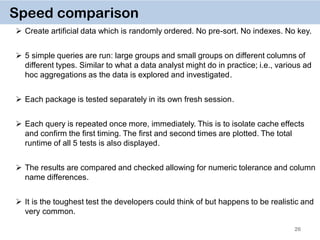
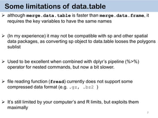
The document discusses the data.table package in R, emphasizing its efficiency and speed for data manipulation tasks, particularly with large datasets. Key features include faster code writing, improved readability, and the ability to efficiently handle operations on extensive data. Limitations and best practices, such as avoiding certain functions and setting keys for optimal performance, are also highlighted.

1. Speeding up
(big) data manipulation with
data.table package
Vasily Tolkachev
Zurich University of Applied Sciences (ZHAW)
Institute for Data Analysis and Process Design (IDP)
vasily.tolkachev@gmail.com
www.idp.zhaw.ch
21.01.2016

2. 2
About me
 Sep. 2014 – Present: Research Assistant in Statistics at
 Sep. 2011 – Aug. 2014: MSc Statistics & Research Assistant at
 Sep. 2008 – Aug. 2011: BSc Mathematical Economics at
 https://ch.linkedin.com/in/vasily-tolkachev-20130b35

3. Motivating example from stackoverflow
3

4. dt = data.table(nuc, key="gene_id")
dt[,list(A = min(start),
B = max(end),
C = mean(pctAT),
D = mean(pctGC),
E = sum(length)),
by = key(dt)]
# gene_id A B C D E
# 1: NM_032291 67000042 67108547 0.5582567 0.4417433 283
# 2: ZZZ 67000042 67108547 0.5582567 0.4417433 283
4
data.table solution
 takes ~ 3 seconds to run !
 easy to program
 easy to understand

5. 5
Huge advantages of data.table
 easier & faster to write the code (no need to write data frame name
multiple times)
 easier to read & understand the code
 shorter code
 fast split-apply-combine operations on large data, e.g. 100GB in RAM
(up to 231 ≈ 2 billion rows in current R version, provided that you have
the RAM)
 fast add/modify/delete columns by reference by group without copies
 fast and smart file reading function ( fread )
 flexible syntax
 easier & faster than other advanced data manipulation packages like
dplyr, plyr, readr.
 backward-compatible with code using data.frame
 named one of the success factors by Kaggle competition winners

6. 6
How to get a lot of RAM
 240 GB of RAM: https://aws.amazon.com/ec2/details/
 6 TB of RAM: http://www.dell.com/us/business/p/poweredge-r920/pd

7. 7
Some limitations of data.table
 although merge.data.table is faster than merge.data.frame, it
requires the key variables to have the same names
 (In my experience) it may not be compatible with sp and other spatial
data packages, as converting sp object to data.table looses the polygons
sublist
 Used to be excellent when combined with dplyr’s pipeline (%>%)
operator for nested commands, but now a bit slower.
 file reading function (fread) currently does not support some
compressed data format (e.g. .gz, .bz2 )
 It’s still limited by your computer’s and R limits, but exploits them
maximally

8. 8
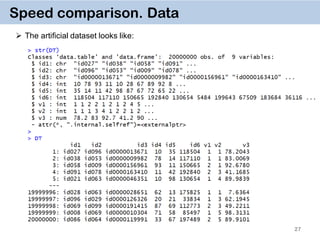
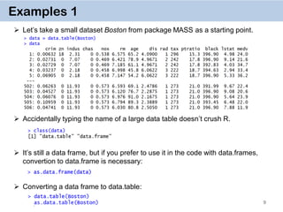
General Syntax
DT[i, j, by]
rows or logical rule
to subset obs.
some function
of the data
To which groups
apply the function
Take DT,
subset rows using i,
then calculate j
grouped by by

9. 9
Examples 1
 Let’s take a small dataset Boston from package MASS as a starting point.
 Accidentally typing the name of a large data table doesn’t crush R.
 It’s still a data frame, but if you prefer to use it in the code with data.frames,
convertion to data.frame is necessary:
 Converting a data frame to data.table:

10.  To get a data.table, use list()  The usual data.frame style is done
with with = FALSE
10
Examples 2
 Subset rows from 11 to 20:
 In this case the result is a vector:
comma not needed when subsetting rows
quotes not needed for variable names

11. 11
Examples 3
 Find all rows where tax variable is equal to 216:
 Find the range of crim (criminality) variable:
 Display values of rad (radius) variable:
 Add a new variable with :=
 i.e. we defined a new factor variable(rad.f) in the data table from the integer
variable radius (rad), which describes accessibility to radial highways.
Tip: with with = FALSE,
you could also select
all columns between some two:

12. 12
Examples 4
 Compute mean of house prices for every level of rad.f:
 Recall that j argument is a function, so in this case it’s a function calling a
variable medv:
 Below it’s a function which is equal to 5:
Here’s the standard way
to select 5th variable

13. 13
Examples 5
 Select several variables Or equivalently:
(result is a data.table)
 Compute several functions:
 Compute these functions for groups (levels) of rad.f:

14. 14
Examples 6
 Compute functions for every level of rad.f and return a data.table with column
names:
 Add many new variables with `:=`().
If a variable attains only a single value, copy it for each observation:
 Updating or deletion of old variables/columns is done the same way

15. 15
Examples 7
 Compute a more complicated function for groups. It’s a weighted mean of house
prices, with dis (distances to Boston employment centers) as weights:
 Dynamic variable creation. Now let’s create a variable of weighted means
(mean_w), and then use it to create a variable for weighted standard deviation
(std_w).

16. 16
Examples 8
 What if variable names are too long and you have a non-standard function where
they are used multiple times?
 Of course, it’s possible to change variable names, do the analysis and then return
to the original names, but if this isn’t an option, one needs to use a list for variable
names .SD, and the variables are specified in.SDcols:
give variable names here
use these instead of variable names

17. 17
Examples 9
 Multiple expressions in j could be handled with { }:

18. 18
Examples 10
 Hence, a separate data.table with dynamically created variables can be done by
 Changing a subset of observations. Let’s create another factor variable crim.f
with 3 levels standing for low, medium and severe crime rates per capita:

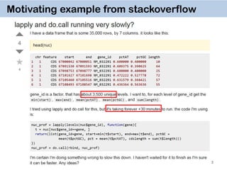
19. 19
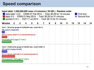
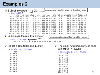
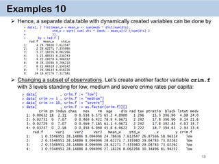
Examples 11. Chaining
DT[i, j, by][i, j, by]
 It’s a very powerful way of doing multiple operations in one command
 The command for crim.f on the previous slide can thus be done by
 Or in one go:
data[…, …][…, …][…, …][…, …]

20. 20
Examples 12
 Now that we have 2 factor variables, crim.f and rad.f, we can also apply
functions in j on two groups:
 It appears that there is one remote district with severe crime rates.
 .N function counts the number observations in a group:

21. 21
Examples 13
 Another useful function is .SD which contains values of all variables except the
one used for grouping:
 Use setnames() and setcolorder() functions to change column names or
reorder them:

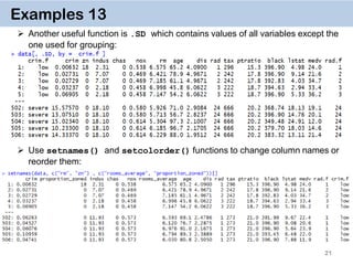
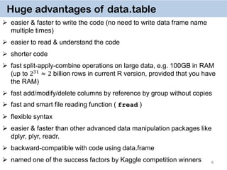
22. 22
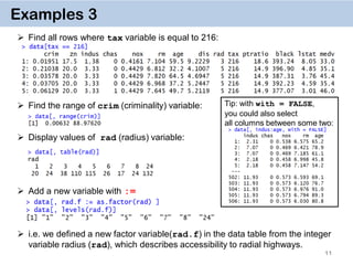
Examples 14. Key on one variable
 The reason why data.table works so fast is the use of keys. All observations are
internally indexed by the way they are stored in RAM and sorted using Radix sort.
 Any column can be set as a key (list & complex number classes not supported),
and duplicate entries are allowed.
 setkey(DT, colA)introduces an index for column A and sorts the data.table by
it increasingly. In contrast to data.frame style, this is done without extra copies and
with a very efficient memory use.
 After that it’s possible to use
binary search by providing index values directly data[“1”], which is 100-
1000… times faster than
vector scan data[rad.f == “1”]
 Setting keys is necessary for joins and significantly speeds up things for big data.
However, it’s not necessary for by = aggregation.

23. 23
Examples 15. Keys on multiple variables
 Any number of columns can be set as key using setkey(). This way rows can
be selected on 2 keys.
 setkey(DT, colA, colB)introduces indexes for both columns and sorts the
data.table by column A, then by column B within each group of column A:
 Then binary search on two keys is

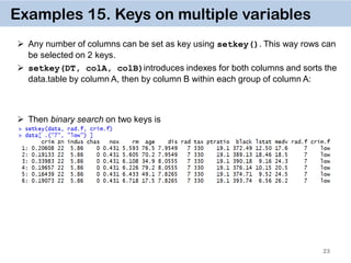
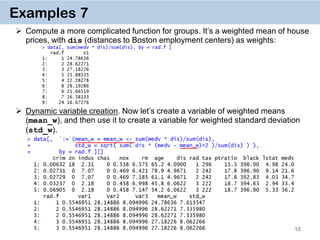
24. 24
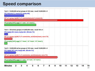
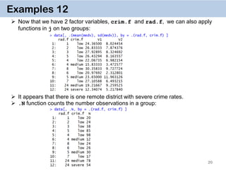
Vector Scan vs. Binary Search
 The reason vector scan is so inefficient is that is searches first for entries “7” in
rad.f variable row-by-row, then does the same for crim.f, then takes element-
wise intersection of logical vectors.
 Binary search, on the other hand, searches already on sorted variables, and
hence cuts the number of observations by half at each step.
 Since rows of each column of data.tables have corresponding locations in RAM
memory, the operations are performed in a very cache efficient manner.
 In addition, since the matching row indices are obtained directly without having to
create huge logical vectors (equal to the number of rows in a data.table), it is quite
memory efficient as well.
Vector Scan Binary search
data[rad.f ==“7” & crim.f == “low”]
setkey(data, rad.f, crim.f)
data[ .(“7”, “low")]
𝑂(𝑛) 𝑂(log⁡( 𝑛))

25. 25
What to avoid
 Avoid read.csv function which takes hours to read in files > 1 Gb. Use fread
instead. It’s a lot smarter and more efficient, e.g. it can guess the separator.
 Avoid rbind which is again notoriously slow. Use rbindlist instead.
 Avoid using data.frame’s vector scan inside data.table:
data[ data$rad.f == "7" & data$crim.f == "low", ]
(even though data.table’s vector scan is faster than data.frame’s vector scan, this
slows it down.)
 In general, avoid using $ inside the data.table, whether it’s for subsetting, or
updating some subset of the observations:
data[ data$rad.f == "7", ] = data[ data$rad.f == "7", ] + 1
 For speed use := by group, don't transform() by group or cbind() afterwards
 data.table used to work with dplyr well, but now it is usually slow:
data %>% filter(rad == 1)

26. 26
Speed comparison
 Create artificial data which is randomly ordered. No pre-sort. No indexes. No key.
 5 simple queries are run: large groups and small groups on different columns of
different types. Similar to what a data analyst might do in practice; i.e., various ad
hoc aggregations as the data is explored and investigated.
 Each package is tested separately in its own fresh session.
 Each query is repeated once more, immediately. This is to isolate cache effects
and confirm the first timing. The first and second times are plotted. The total
runtime of all 5 tests is also displayed.
 The results are compared and checked allowing for numeric tolerance and column
name differences.
 It is the toughest test the developers could think of but happens to be realistic and
very common.

27. 27
Speed comparison. Data
 The artificial dataset looks like:

28. 28
Speed comparison

29. 29
Speed comparison

30. 30
References
 Matt Dowle’s data.table git account with newest vignettes.
https://github.com/Rdatatable/data.table/wiki
 Matt Dowle’s presentations & conference videos.
https://github.com/Rdatatable/data.table/wiki/Presentations
 Official introduction to data.table:
https://github.com/Rdatatable/data.table/wiki/Getting-started
 Why to set keys in data.table:
http://stackoverflow.com/questions/20039335/what-is-the-purpose-of-setting-a-
key-in-data-table
 Performance comparisons to other packages:
https://github.com/Rdatatable/data.table/wiki/Benchmarks-%3A-Grouping
 Comprehensive data.table summary sheet:
https://s3.amazonaws.com/assets.datacamp.com/img/blog/data+table+cheat+she
et.pdf
 An unabridged comparison of dplyr and data.table:
http://stackoverflow.com/questions/21435339/data-table-vs-dplyr-can-one-do-
something-well-the-other-cant-or-does-poorly/27840349#27840349

31. Thanks a lot for
your attention and interest!