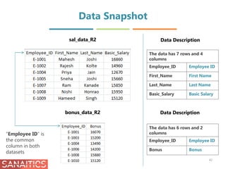
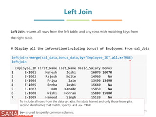
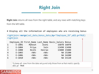
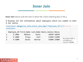
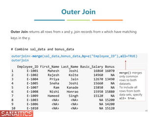
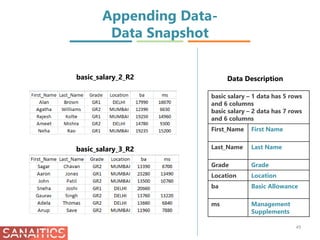
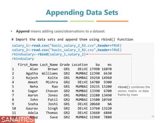
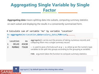
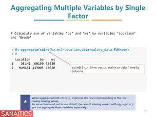
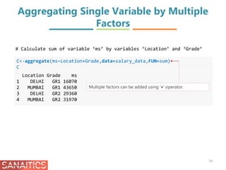
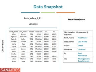
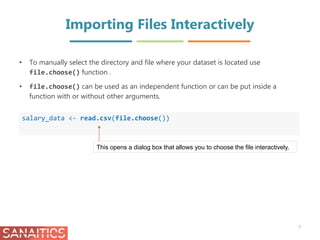
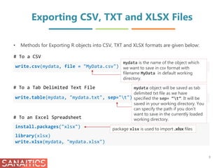
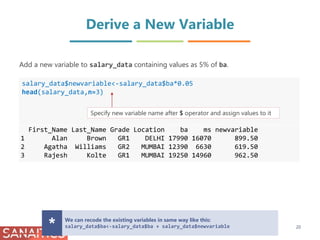
The document discusses importing and exporting data in R. It describes how to import data from CSV, TXT, and Excel files using functions like read.table(), read.csv(), and read_excel(). It also describes how to export data to CSV, TXT, and Excel file formats using write functions. The document also demonstrates how to check the structure and dimensions of data, modify variable names, derive new variables, and recode categorical variables in R.


![Dimension of Data and Names of the
Columns
dim(salary_data)
[1] 12 6
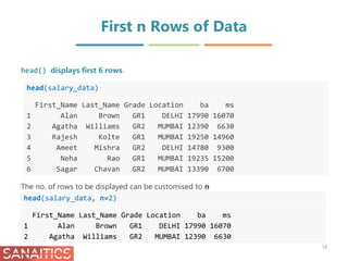
dim() displays the no. of rows and columns in data.:
# Retrieve the Dimension of your data using dim()
Data contains 12 rows and 6 columns
OR
nrow() and ncol() can be used separately to know no. of rows
and columns.
names(salary_data)
[1] "First_Name" "Last_Name" "Grade" "Location"
[5] "ba" "ms"
# Get the Names of the columns using names()
10
names() displays the names of the columns of data](https://image.slidesharecdn.com/datamanagementinr-170925105148/85/Data-Management-in-R-10-320.jpg)
![Check the Levels
levels(salary_data$Grade)
[1] "GR1" "GR2"
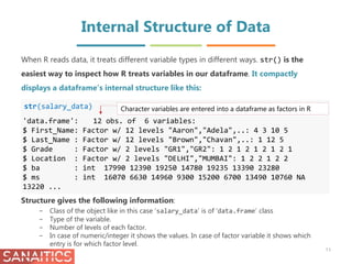
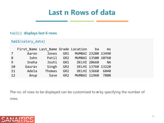
Our data has 4 factor variables. A factor is a categorical variable that can take only one
of a fixed, finite set of possibilities. Those possible categories are the levels. We can
check the levels using levels() function
12
You can assign individual levels, for example:
levels(salary_data$Grade)[1]<-"G1"
or as a group, for example:
levels(salary_data$Grade)<-c("G1", "G2")](https://image.slidesharecdn.com/datamanagementinr-170925105148/85/Data-Management-in-R-12-320.jpg)
![Number of Missing Observations
nmiss<-sum(is.na(salary_data$ms))
nmiss
[1] 1
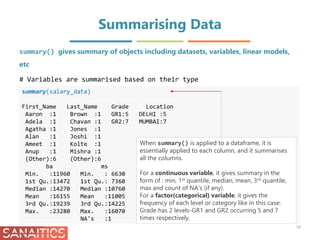
In R missing data are usually recorded as NA.
# Check the number of missing values in the data.
$ operator after a data frame object helps in selecting a column
from the data frame.
is.na() returns a logical vector giving information about missing
values.
Here sum() displays the sum of missing observations.
13](https://image.slidesharecdn.com/datamanagementinr-170925105148/85/Data-Management-in-R-13-320.jpg)

![Change Variable Names – rename()
install.packages("reshape")
library(reshape)
salary_data<-rename(salary_data,c(ba="basic allowance"))
names(salary_data)
[1] "First_Name" "Last_Name" "Grade"
[4] "Location" "basic allowance" "ms"
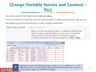
Another way of renaming columns is by using package reshape.
rename() uses name of the data object and (old name="new name").
The result need to be saved in an object because rename() doesn’t modify the object directly.
You can rename multiple column names like this:
salary_data<-rename(salary_data, c(ba="basic allowance", ms="management
supplements"))
Alternative way to change column names:
names(salary_data)[names(salary_data)=="ba"] <- "basic allowance"
Note that this modifies salary_data directly; i.e. you don’t have to save the result
back into salary_data.
*
# Install and load package reshape
# Use rename() from package reshape to change the column names
19](https://image.slidesharecdn.com/datamanagementinr-170925105148/85/Data-Management-in-R-19-320.jpg)
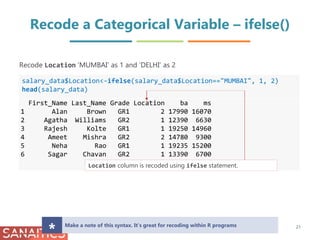
![Recode a Continuous Variable into
Categorical Variable – ifelse()
salary_data$category<-ifelse(salary_data$ba <14000, "Low",
ifelse(salary_data$ba <19000, "Medium", "High"))
head(salary_data)
First_Name Last_Name Grade Location ba ms category
1 Alan Brown GR1 2 17990 16070 Medium
2 Agatha Williams GR2 1 12390 6630 Low
3 Rajesh Kolte GR1 1 19250 14960 High
4 Ameet Mishra GR2 2 14780 9300 Medium
5 Neha Rao GR1 1 19235 15200 High
6 Sagar Chavan GR2 1 13390 6700 Low
class(salary_data$category)
[1] "character"
Categorise the employees on the basis of their ba in three categories, namely, Low,
Medium and High
22
Nested ifelse statement is used. Alternate command using cut() function
salary_data$category<-
cut(salary_data$ba,breaks=c(0,13999,18999,Inf),labels=c("Low","Medium","High"))
Note that column category is of character type. You
will have to convert it to a factor using as.factor()](https://image.slidesharecdn.com/datamanagementinr-170925105148/85/Data-Management-in-R-22-320.jpg)
![Remove Columns from a Data Frame
salary_data$Last_Name<-NULL
head(salary_data)
First_Name Grade Location ba ms newvariable
1 Alan GR1 DELHI 17990 16070 899.50
2 Agatha GR2 MUMBAI 12390 6630 619.50
3 Rajesh GR1 MUMBAI 19250 14960 962.50
4 Ameet GR2 DELHI 14780 9300 739.00
5 Neha GR1 MUMBAI 19235 15200 961.75
6 Sagar GR2 MUMBAI 13390 6700 669.50
To remove a column, set it to NULL
Remove a column Last_Name from salary_data.
To remove columns using integer indexing : salary_data[6]<-NULL
Index is the position of column. It starts from 1.
In this case index number of First_Name is 1, Grade is 2 and so on and so forth.* 23](https://image.slidesharecdn.com/datamanagementinr-170925105148/85/Data-Management-in-R-23-320.jpg)
![Remove Rows from a Data Frame
salary_data[-(2:4),]
First_Name Last_Name Grade Location ba ms
1 Alan Brown GR1 DELHI 17990 16070
5 Neha Rao GR1 MUMBAI 19235 15200
6 Sagar Chavan GR2 MUMBAI 13390 6700
7 Aaron Jones GR1 MUMBAI 23280 13490
8 John Patil GR2 MUMBAI 13500 10760
9 Sneha Joshi GR1 DELHI 20660 NA
10 Gaurav Singh GR2 DELHI 13760 13220
11 Adela Thomas GR2 DELHI 13660 6840
12 Anup Save GR2 MUMBAI 11960 7880
Remove unwanted rows from data using their index no.s. We can use the [] bracket
notation to access the indices of rows and columns like this: [R, C]. Here, the first index
is for Rows and the second is for Columns.
# Remove rows 2, 3 and 4 from salary_data .
24](https://image.slidesharecdn.com/datamanagementinr-170925105148/85/Data-Management-in-R-24-320.jpg)
![Remove Rows from a Data Frame
salary_data[!(salary_data$Location=="MUMBAI"),]
First_Name Last_Name Grade Location ba ms
1 Alan Brown GR1 DELHI 17990 16070
4 Ameet Mishra GR2 DELHI 14780 9300
9 Sneha Joshi GR1 DELHI 20660 NA
10 Gaurav Singh GR2 DELHI 13760 13220
11 Adela Thomas GR2 DELHI 13660 6840
25
Remove only rows which has Location as ‘MUMBAI’
Use negation (!) operator to remove the row which satisfies
the condition.
You can specify multiple conditions like this:
salary_data[!(salary_data$Location=="MUMBAI" &
salary_data$Grade=="GR2"),]](https://image.slidesharecdn.com/datamanagementinr-170925105148/85/Data-Management-in-R-25-320.jpg)

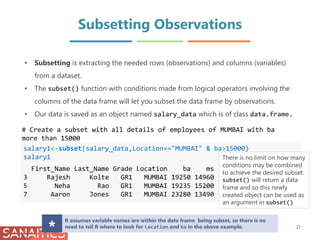
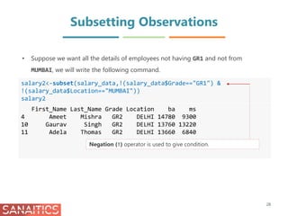
![Row Subsetting
salary_data [5:10, ]
First_Name Last_Name Grade Location ba ms
5 Neha Rao GR1 MUMBAI 19235 15200
6 Sagar Chavan GR2 MUMBAI 13390 6700
7 Aaron Jones GR1 MUMBAI 23280 13490
8 John Patil GR2 MUMBAI 13500 10760
9 Sneha Joshi GR1 DELHI 20660 NA
10 Gaurav Singh GR2 DELHI 13760 13220
# Display rows from 5th to 10th
31
When we only want to subset rows we use the first index and leave the second index blank.
Leaving an index blank indicates that you want to keep all the elements in that dimension.
Use names() to know which column corresponds to which no. in the index. Use colon
notation(:) if rows have consecutive positions.](https://image.slidesharecdn.com/datamanagementinr-170925105148/85/Data-Management-in-R-31-320.jpg)
![Row Subsetting
salary_data[c(1,3,5), ]
First_Name Last_Name Grade Location ba ms
1 Alan Brown GR1 DELHI 17990 16070
3 Rajesh Kolte GR1 MUMBAI 19250 14960
5 Neha Rao GR1 MUMBAI 19235 15200
# Display only selected rows
32
c() can be used to give a list of
row indices if the rows are not in
sequential order](https://image.slidesharecdn.com/datamanagementinr-170925105148/85/Data-Management-in-R-32-320.jpg)
![Column Subsetting
salary5<-salary_data[ ,1:4]
head(salary5)
First_Name Last_Name Grade Location
1 Alan Brown GR1 DELHI
2 Agatha Williams GR2 MUMBAI
3 Rajesh Kolte GR1 MUMBAI
4 Ameet Mishra GR2 DELHI
5 Neha Rao GR1 MUMBAI
6 Sagar Chavan GR2 MUMBAI
# Display columns 1 to 4
33
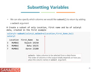
• We can subset variables also using [] bracket notation but now we use the second
index and leave the first index blank. This indicates that we want all the rows for
specific columns.](https://image.slidesharecdn.com/datamanagementinr-170925105148/85/Data-Management-in-R-33-320.jpg)
![Row-Column Subsetting
salary6<-salary_data[c(1,5,8),c(1,2)]
salary6
First_Name Last_Name
1 Alan Brown
5 Neha Rao
8 John Patil
# Display rows 1,5,8 and columns 1 and 2
34
We can also subset the columns by name as in select for subset() like
this:
salary6<-salary_data[c(1,5,8),c(“First_Name”, “Last_Name”)]](https://image.slidesharecdn.com/datamanagementinr-170925105148/85/Data-Management-in-R-34-320.jpg)
![Sorting data in Ascending Order
attach(salary_data)
ba_sorted_1<-salary_data[order(ba),]
ba_sorted_1
First_Name Last_Name Grade Location ba ms
12 Anup Save GR2 MUMBAI 11960 7880
2 Agatha Williams GR2 MUMBAI 12390 6630
6 Sagar Chavan GR2 MUMBAI 13390 6700
8 John Patil GR2 MUMBAI 13500 10760
11 Adela Thomas GR2 DELHI 13660 6840
10 Gaurav Singh GR2 DELHI 13760 13220
4 Ameet Mishra GR2 DELHI 14780 9300
1 Alan Brown GR1 DELHI 17990 16070
5 Neha Rao GR1 MUMBAI 19235 15200
3 Rajesh Kolte GR1 MUMBAI 19250 14960
9 Sneha Joshi GR1 DELHI 20660 NA
7 Aaron Jones GR1 MUMBAI 23280 13490
order() is
used to sort a
vector, matrix
or data frame.
By default, it
sorts in
ascending
order
36
# Sort salary_data by ba in Ascending order
Sorting is storage of data in sorted order, it can be in ascending or descending
order.](https://image.slidesharecdn.com/datamanagementinr-170925105148/85/Data-Management-in-R-36-320.jpg)
![ba_sorted_2<-salary_data[order(-ba),]
ba_sorted_2
First_Name Last_Name Grade Location ba ms
7 Aaron Jones GR1 MUMBAI 23280 13490
9 Sneha Joshi GR1 DELHI 20660 NA
3 Rajesh Kolte GR1 MUMBAI 19250 14960
5 Neha Rao GR1 MUMBAI 19235 15200
1 Alan Brown GR1 DELHI 17990 16070
4 Ameet Mishra GR2 DELHI 14780 9300
10 Gaurav Singh GR2 DELHI 13760 13220
11 Adela Thomas GR2 DELHI 13660 6840
8 John Patil GR2 MUMBAI 13500 10760
6 Sagar Chavan GR2 MUMBAI 13390 6700
2 Agatha Williams GR2 MUMBAI 12390 6630
12 Anup Save GR2 MUMBAI 11960 7880
Sorting data in Descending Order
37
# Sort salary_data by ba in Descending order
The ‘-’ sign before a
numeric column
reverses the default
order.
Alternatively , here
you can add
decreasing=TRUE](https://image.slidesharecdn.com/datamanagementinr-170925105148/85/Data-Management-in-R-37-320.jpg)
![Sorting by Factor Variable
gr_sorted<-salary_data[order(Grade),]
gr_sorted
First_Name Last_Name Grade Location ba ms
1 Alan Brown GR1 DELHI 17990 16070
3 Rajesh Kolte GR1 MUMBAI 19250 14960
5 Neha Rao GR1 MUMBAI 19235 15200
7 Aaron Jones GR1 MUMBAI 23280 13490
9 Sneha Joshi GR1 DELHI 20660 NA
2 Agatha Williams GR2 MUMBAI 12390 6630
4 Ameet Mishra GR2 DELHI 14780 9300
6 Sagar Chavan GR2 MUMBAI 13390 6700
8 John Patil GR2 MUMBAI 13500 10760
10 Gaurav Singh GR2 DELHI 13760 13220
11 Adela Thomas GR2 DELHI 13660 6840
12 Anup Save GR2 MUMBAI 11960 7880
• Sort data by column with characters / factors
Note that by default
order() sorts in
ascending order
38
# Sort salary_data by Grade](https://image.slidesharecdn.com/datamanagementinr-170925105148/85/Data-Management-in-R-38-320.jpg)
![Sorting Data by Multiple Variables
grba_sorted<-salary_data[order(Grade,ba),]
grba_sorted
First_Name Last_Name Grade Location ba ms
1 Alan Brown GR1 DELHI 17990 16070
5 Neha Rao GR1 MUMBAI 19235 15200
3 Rajesh Kolte GR1 MUMBAI 19250 14960
9 Sneha Joshi GR1 DELHI 20660 NA
7 Aaron Jones GR1 MUMBAI 23280 13490
12 Anup Save GR2 MUMBAI 11960 7880
2 Agatha Williams GR2 MUMBAI 12390 6630
6 Sagar Chavan GR2 MUMBAI 13390 6700
8 John Patil GR2 MUMBAI 13500 10760
11 Adela Thomas GR2 DELHI 13660 6840
10 Gaurav Singh GR2 DELHI 13760 13220
4 Ameet Mishra GR2 DELHI 14780 9300
• Sort data by giving multiple columns; one column with characters / factors and
one with numerals
39
# Sort salary_data by Grade and ba
Here, data is first
sorted in increasing
order of Grade then
ba.](https://image.slidesharecdn.com/datamanagementinr-170925105148/85/Data-Management-in-R-39-320.jpg)
![Multiple Variables & Multiple Ordering
Levels
grms_sorted<-salary_data[order(Grade,decreasing=TRUE,-ms),]
grms_sorted
First_Name Last_Name Grade Location ba ms
2 Agatha Williams GR2 MUMBAI 12390 6630
6 Sagar Chavan GR2 MUMBAI 13390 6700
11 Adela Thomas GR2 DELHI 13660 6840
12 Anup Save GR2 MUMBAI 11960 7880
4 Ameet Mishra GR2 DELHI 14780 9300
8 John Patil GR2 MUMBAI 13500 10760
10 Gaurav Singh GR2 DELHI 13760 13220
7 Aaron Jones GR1 MUMBAI 23280 13490
3 Rajesh Kolte GR1 MUMBAI 19250 14960
5 Neha Rao GR1 MUMBAI 19235 15200
1 Alan Brown GR1 DELHI 17990 16070
9 Sneha Joshi GR1 DELHI 20660 NA
• Sort data by giving multiple columns; one column with characters / factors and
one with numerals and multiple ordering levels
40
# Sort salary_data by Grade in Descending order and then by ms in
# Ascending order
Here, data is sorted by
Grade in descending
order and ms in
ascending order.
By default missing
values in data are put
last.
You can put it first by
adding an argument
na.last=FALSE in
order().](https://image.slidesharecdn.com/datamanagementinr-170925105148/85/Data-Management-in-R-40-320.jpg)