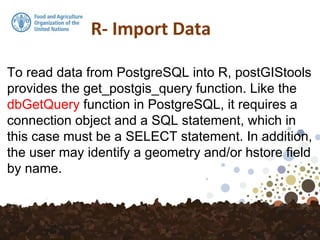
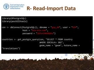
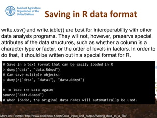
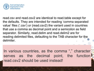
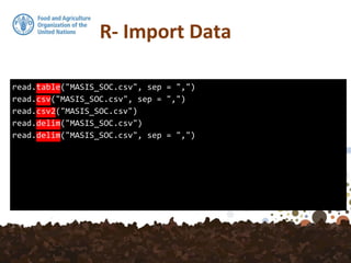
The document discusses various functions for reading data into R from files and databases, as well as writing data out of R. It describes read.csv and read.csv2 for reading comma separated value (CSV) files, with read.csv2 handling CSV formats with commas as decimal separators. It also covers reading from databases using functions like get_postgis_query and reading/writing directly from/to R using dump and source. Writing data out can be done with write.csv or to a format preserved R data with dump.

5. read.csv and read.csv2 are identical to read.table except for
the defaults. They are intended for reading ‘comma separated
value’ files (‘.csv’) or (read.csv2) the variant used in countries
that use a comma as decimal point and a semicolon as field
separator. Similarly, read.delim and read.delim2 are for
reading delimited files, defaulting to the TAB character for the
delimiter.
In various countries, as the comma “,” character
serves as the decimal point, the function
read.csv2 should be used instead!

6. read.table("MASIS_SOC.csv", sep = ",")
read.csv("MASIS_SOC.csv", sep = ",")
read.csv2("MASIS_SOC.csv")
read.delim("MASIS_SOC.csv")
read.delim("MASIS_SOC.csv", sep = ",")

7. read.table("MASIS_SOC.csv", sep = ",")
read.csv("MASIS_SOC.csv", sep = ",")
read.csv2("MASIS_SOC.csv")
read.delim("MASIS_SOC.csv")
read.delim("MASIS_SOC.csv", sep = ",")

8. Unless you take any special action, read.table() reads all the
columns as character vectors and then tries to select a
suitable class for each variable in the data frame. It tries in
logical, integer, numeric and complex. If all of these fail, the
variable is converted to a factor.
More about Factors: https://www.stat.berkeley.edu/classes/s133/factors.html

9. > is.na(SOC)
Id UpperDepth LowerDepth SOC Lambda tsme Region
[1,] FALSE FALSE FALSE FALSE FALSE FALSE FALSE
[2,] FALSE FALSE FALSE FALSE FALSE FALSE FALSE
[3,] FALSE FALSE FALSE FALSE FALSE FALSE FALSE
[4,] FALSE FALSE FALSE FALSE FALSE FALSE FALSE
[5,] FALSE FALSE FALSE FALSE FALSE FALSE FALSE
[6,] FALSE FALSE FALSE FALSE FALSE FALSE FALSE
[7,] FALSE FALSE FALSE FALSE FALSE FALSE FALSE
[8,] FALSE FALSE FALSE FALSE FALSE FALSE FALSE
[9,] FALSE FALSE FALSE FALSE FALSE FALSE FALSE
[10,] FALSE FALSE FALSE FALSE FALSE FALSE FALSE
...

10. > anyNA(SOC)
[1] TRUE
> sum(is.na(SOC$SOC))
[1] 1

11. Importing from other statistical systems
install.packages("foreign")
library(foreign)
stata <- read.dta(“salary.dta”)
spss <- read.spss(“salary.sav”, to.data.frame=TRUE)
sasxport <- read.xport(“salary.xpt”)
epiinfo <- read.epiinfo(“salary.rec”) …
Note: The foreign package is in the standard distribution. It
handles import and export of data.

12. Reading Data from Web
> read.table("http://www.cdc.noaa.gov/data/correlation/nao.data",skip=1,
nrow=62, na.strings="-99.90")
V1 V2 V3 V4 V5 V6 V7 V8 V9 V10 V11 V12 V13
1 1948 NA NA NA NA NA NA NA NA NA NA NA NA
2 1949 NA NA NA NA NA NA NA NA NA NA NA NA
3 1950 0.56 0.01 -0.78 0.65 -0.50 0.25 -1.23 -0.19 0.39 1.43 -1.46 -1.03
4 1951 -0.42 0.35 -1.47 -0.38 -0.50 -1.35 1.39 -0.41 -1.18 2.54 -0.54 1.13
5 1952 0.57 -1.38 -1.97 0.95 -0.99 -0.10 -0.06 -0.49 -0.38 -0.28 -1.32 -0.49
6 1953 -0.12 -1.00 -0.45 -1.96 -0.56 1.41 0.43 -1.04 -0.19 1.95 0.96 -0.52
7 1954 -0.08 0.40 -1.27 1.31 -0.03 0.06 -0.57 -2.57 -0.28 1.16 0.29 0.55
8 1955 -2.65 -1.71 -0.96 -0.60 -0.26 -0.80 1.78 1.25 0.46 -1.09 -1.49 0.07
9 1956 -0.76 -1.71 -0.46 -1.30 2.10 0.41 -0.72 -1.89 0.38 1.47 0.40 0.00

13. Reading Data from Web
> read.table("http://www.cdc.noaa.gov/data/correlation/nao.data",skip=1,
nrow=62)
V1 V2 V3 V4 V5 V6 V7 V8 V9 V10 V11 V12 V13
1 1948 -99.90 -99.90 -99.90 -99.90 -99.90 -99.90 -99.90 -99.90 -99.90 -99.90 -99.90 -99.90
2 1949 -99.90 -99.90 -99.90 -99.90 -99.90 -99.90 -99.90 -99.90 -99.90 -99.90 -99.90 -99.90
3 1950 0.56 0.01 -0.78 0.65 -0.50 0.25 -1.23 -0.19 0.39 1.43 -1.46 -1.03
4 1951 -0.42 0.35 -1.47 -0.38 -0.50 -1.35 1.39 -0.41 -1.18 2.54 -0.54 1.13
5 1952 0.57 -1.38 -1.97 0.95 -0.99 -0.10 -0.06 -0.49 -0.38 -0.28 -1.32 -0.49
6 1953 -0.12 -1.00 -0.45 -1.96 -0.56 1.41 0.43 -1.04 -0.19 1.95 0.96 -0.52
7 1954 -0.08 0.40 -1.27 1.31 -0.03 0.06 -0.57 -2.57 -0.28 1.16 0.29 0.55
8 1955 -2.65 -1.71 -0.96 -0.60 -0.26 -0.80 1.78 1.25 0.46 -1.09 -1.49 0.07
9 1956 -0.76 -1.71 -0.46 -1.30 2.10 0.41 -0.72 -1.89 0.38 1.47 0.40 0.00
10 1957 0.71 -0.32 -1.73 0.39 -0.68 -0.42 -1.16 -0.83 -1.47 1.95 0.63 0.02

14. Reading Data from Web
> read.table("http://www.cdc.noaa.gov/data/correlation/nao.data")
Error in scan(file = file, what = what, sep = sep, quote = quote, dec =
dec, : line 1 did not have 13 elements

15. PostGIS Spatial Databases
PostGIS is a spatial database extender for
PostgreSQL object-relational database. It adds
support for geographic objects allowing location
queries to be run in SQL.

16. PostGIS Spatial Databases
PostGIS is a spatial database extender for
PostgreSQL object-relational database. It adds
support for geographic objects allowing location
queries to be run in SQL.

17. To read data from PostgreSQL into R, postGIStools
provides the get_postgis_query function. Like the
dbGetQuery function in PostgreSQL, it requires a
connection object and a SQL statement, which in
this case must be a SELECT statement. In addition,
the user may identify a geometry and/or hstore field
by name.

18. library(RPostgreSQL)
library(postGIStools)
con <- dbConnect(PostgreSQL(), dbname = "gsp_db", user = "GSP",
host = "bla-bla.com",
password = "587vn34m98dhu")
countries <- get_postgis_query(con, "SELECT * FROM country
WHERE SOCStck> 102",
geom_name = "geom", hstore_name =
"translations")

19. > write.csv(SOC,file = "SOCData.csv")
The easiest way to do this is to use write.csv(). By default, write.
csv() includes row names, but these are usually unnecessary and
may cause confusion.

20. > write.csv(SOC,file = "SOCData.csv")
The easiest way to do this is to use write.csv(). By default, write.
csv() includes row names, but these are usually unnecessary and
may cause confusion.

21. # Save in a text format that can be easily loaded in R
> dump("data", "data.Rdmpd")
# Can save multiple objects:
> dump(c("data", "data1"), "data.Rdmpd")
# To load the data again:
source("data.Rdmpd")
# When loaded, the original data names will automatically be used.
write.csv() and write.table() are best for interoperability with other
data analysis programs. They will not, however, preserve special
attributes of the data structures, such as whether a column is a
character type or factor, or the order of levels in factors. In order to
do that, it should be written out in a special format for R.
More on: Rdmpd: http://www.cookbook-r.com/Data_input_and_output/Writing_data_to_a_file/

22. # Save in a text format that can be easily loaded in R
> dump("data", "data.Rdmpd")
# Can save multiple objects:
> dump(c("data", "data1"), "data.Rdmpd")
# To load the data again:
source("data.Rdmpd")
# When loaded, the original data names will automatically be used.
write.csv() and write.table() are best for interoperability with other
data analysis programs. They will not, however, preserve special
attributes of the data structures, such as whether a column is a
character type or factor, or the order of levels in factors. In order to
do that, it should be written out in a special format for R.
More on: Rdmpd: http://www.cookbook-r.com/Data_input_and_output/Writing_data_to_a_file/