R is a free and open-source language and environment for statistical computing and graphics. It contains a variety of statistical and graphical techniques built in. This document provides an introduction to using R, including how to import and manage data, perform basic analyses and visualizations, and save scripts. It covers topics such as importing data from CSV and text files, creating and subsetting data frames, recoding variables, sorting and merging data, and using basic functions.

1. GET STARTED IN R
Module I
1

2. What is R?
• A language and environment for statistical computing
and graphics
• Wide variety of statistical & graphical techniques built in
• Free and Open Source software
• Compiles and runs on a wide variety of UNIX platforms,
Windows and MacOS
2

3. R Environment
• Most functionality through built in functions
• Basic functions available by default
• Other functions contained in packages that can be
attached
• All datasets created in the session are in Memory
• Output can be used as input to other functions
3

4. R-CRAN
• The Comprehensive R Archive Network
• A network of global web servers storing identical, up-to-
date, versions of code and documentation for R
• Use the CRAN mirror nearest to you to download R
setup at a faster speed
• http://cran.r-project.org/
4

5. Introduction to R and User Interface (UI)
5

6. The R-UI
6
The R console
-- Type in the command
-- Press enter
-- See the output

7. Create Your Data Set
x<-c(12,23,45)
y<-c(13,21,6) Create vectors x, y, z on R Console
z<-c("a","b","c")
data1<-data.frame(x,y,z) Combine them in a table
data1 Type data name for output
7

8. Your data in Table mode
edit(data1)
Edit your table, add new values & close the window to save your
updates
8

9. Export your updated table
write.csv (data1,file.choose())
Select the path, name your file and click save
9

10. Data Set types
10
Vector 1 dimension
All elements have the same data
types
Numeric
Character
Logic
Factor
Matrix 2 dimensions
Array
2 or more
dimensions
Data frame 2 dimensions
Table-like data object allowing
different data types for different
columns
List
Collection of data objects, each element of a list is a data
object

11. Useful In-Built Functions
min(data1$x) Use $ sign after data set name to use specific columns
max(data1$y) length(data1$x)
mean(data1$y)
levels(data1$z) Gives a list of unique categories in the data
11

12. Save Your Script
Open a new script, write commands, execute using F5 key. Save the file at a desired
folder. Helps to save the script for a later use.
12

13. R Workspace
• Objects that you create during an R session are hold
in memory, the collection of objects that you
currently have is called the workspace
• This workspace is not saved on disk unless you tell R
to do so
• This means that your objects are lost when you close
R and not save the objects, or worse when R or your
system crashes on you during a session
13

14. R Workspace
• If you have saved a workspace image and you start R
the next time, it will restore the workspace
• So all your previously saved objects are available
again
• You can also explicitly load a saved workspace i.e.,
that could be the workspace image of someone else
• Go the `File' menu and select `Load workspace'
14

15. R Workspace
Display last 25 commands
history()
Display all previous commands
history(max.show=Inf)
Save your command history to a file. Default is ".Rhistory"
savehistory(file="myfile")
Recall your command history. Default is ".Rhistory"
loadhistory(file="myfile")
15

16. Types of Variables
• Type: Logical, integer, double, complex, character,
factor or raw
• Type conversion functions have the naming
convention
as.xxx
• For example, as.integer(3.2) returns the integer 3,
and as.character(3.2) returns the string "3.2".
16

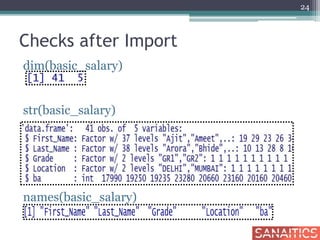
17. Factors
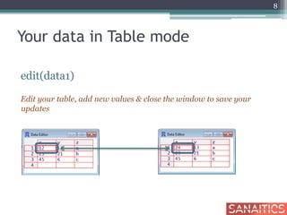
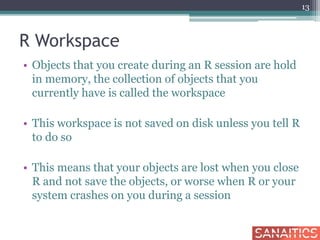
• Tell R that a variable is nominal by making it a
factor
• The factor stores the nominal values as a vector of
integers in the range [ 1... k ] (where k is the number
of unique values in the nominal variable), and an
internal vector of character strings (the original
values) mapped to these integers
• An ordered factor is used to represent an ordinal
variable
17

18. Factors
• R will treat factors as nominal variables and ordered
factors as ordinal variables in statistical procedures
and graphical analyses
• You can use options in the factor( ) and ordered( )
functions to control the mapping of integers to
strings (overriding the alphabetical ordering)
18

19. Help in R
• If you know the topic but not the exact function
Help.search(“topic”)
• If you know the exact function
Help(functionname)
19

20. In-Memory Computing
• Storage of information in the main RAM of
dedicated servers rather than in complicated
relational databases operating on comparatively
slow disk drives
• Helps business customers, including retailers,
banks and utilities, to quickly detect patterns,
analyze massive data volumes on the fly, and
perform their operations quickly
20

21. Import .csv Data File
basic_salary<-read.table(“C:/Users/Documents/R/BASIC
SALARY DATA.csv", header=TRUE, sep=",")
• Command requires the file path separated by a /
• header=TRUE if there are row labels
21

22. Data Imported
Use Head function to get an idea about how your data looks like
head(basic_salary)
22

23. Manual Import
basic_salary<-read.table(file.choose(), header=TRUE ,
sep=",")
Select file of interest and click open to import
23

24. Checks after Import
dim(basic_salary)
str(basic_salary)
names(basic_salary)
24

25. Importing .txt File
#importing a text file having dlm = “blank/space”
sample1<-read.table(file.choose(),header=T)
sample1
#importing a comma separated text file
new<-read.table(file.choose(), header=T, sep=",")
new
#another mehod for importing a comma separated text
file
new1<-read.csv(file.choose(),header=T)
new1
25

26. Data Management: Creating Subsets
26

27. Using Indices
• Row level sub setting: display some selected
rows
• Sub setting by putting condition on observations
• Column level sub setting: display some selected
columns
• Sub setting by putting condition on variable
names
• Display selected rows for selected columns
• Sub setting by putting conditions on variables
and observations
27

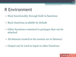
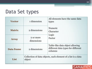
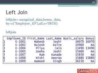
28. Row Sub-Setting
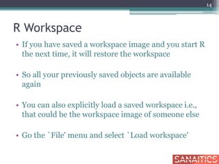
basic_salary[c(5:10), ] Display rows from 5th to 10th
28

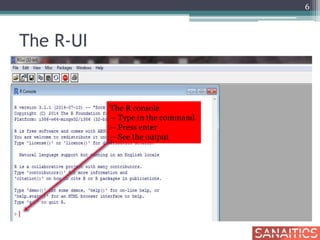
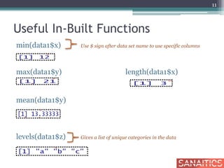
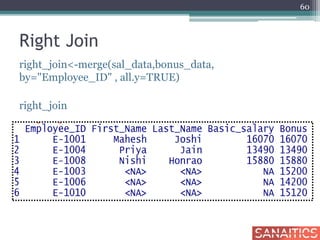
29. Row Sub-Setting
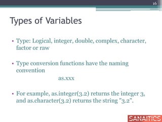
basic_salary[c(1,3,5,8), ] Display only selected rows
29

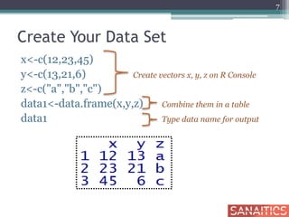
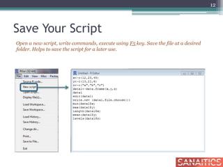
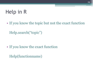
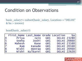
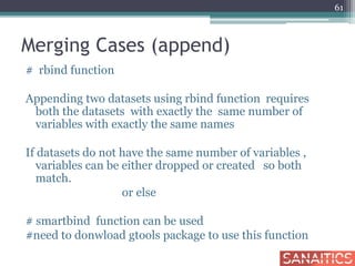
30. Condition on Observations
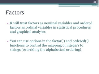
basic_salary1 <- basic_salary[basic_salary$Location
==“DELHI” & basic_salary$ba > 20000, ]
head(basic_salary1)
30

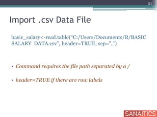
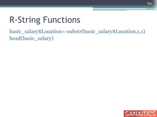
31. More than one value of Variable
basic_salary2 <-basic_salary[basic_salary$Location %in%
c("MUMBAI"),]
head(basic_salary2)
31

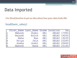
32. Column Sub-Setting
basic_salary3<-basic_salary[ , 1:2]
head(basic_salary3)
32

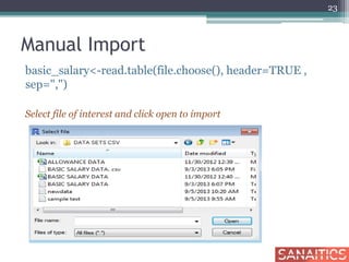
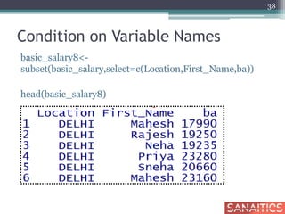
33. Condition on Variable Names
basic_salary4 <- basic_salary[ ,c("First_Name","Location",
"ba")]
head(basic_salary4)
33

34. Selected Rows for Selected Columns
basic_salary5<-basic_salary[c(1,5,8,4), c(1,2)]
basic_salary5
34

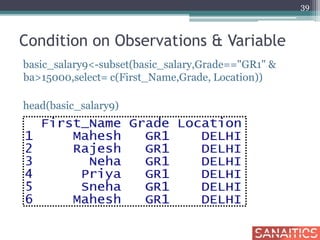
35. Condition on Variables & Observations
basic_salary6<-basic_salary[basic_salary$Grade=="GR1"
& basic_salary$ba >15000 , c("First_Name","Location",
"ba") ]
head(basic_salary6)
35

36. Subset Function
• Condition on observations
• Condition on variable names
• Condition on observations and variable names
36

37. Condition on Observations
basic_salary7<-subset(basic_salary, Location=="DELHI"
& ba > 20000)
head(basic_salary7)
37

38. Condition on Variable Names
basic_salary8<-
subset(basic_salary,select=c(Location,First_Name,ba))
head(basic_salary8)
38

39. Condition on Observations & Variable
basic_salary9<-subset(basic_salary,Grade=="GR1" &
ba>15000,select= c(First_Name,Grade, Location))
head(basic_salary9)
39

40. Using Head Function
head(basic_salary, n=5)
40

41. Using Tail Function
tail(basic_salary, n=5)
41

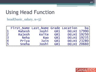
42. Using Split Function
basic_salary10<-
split(basic_salary,basic_salary$Location)
delhi_salary<-data.frame(basic_salary10[1])
head(delhi_salary)
42

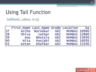
43. Using Split Function
mumbai_salary<-data.frame(basic_salary10[2])
head(mumbai_salary,5)
43

44. Delete Cases
basic_salary11<-
basic_salary[!(basic_salary$Grade=="GR1") &
!(basic_salary$Location=="MUMBAI"), ]
basic_salary11
44

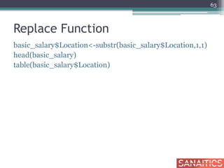
45. Delete Cases
basic_salary12<-basic_salary[ !(basic_salary$ba>14500), ]
basic_salary12
45

46. Recoding Based on Quartiles
brk1<-with(basic_salary,quantile(basic_salary$ba,probs<-
seq(0,1,0.25)))
brk1
basic_salary13<-within(basic_salary,salary_quartile<-
cut(basic_salary$ba,breaks=brk1,labels=1:4,include.lowest
=TRUE))
46

47. Recoding Based on Quartiles
head(basic_salary13)
47

48. Recoding Based on Deciles
brk2<-with(basic_salary,quantile(basic_salary$ba,
probes<-seq(0,1,0.10)))
brk2
basic_salary14<-within(basic_salary,salary_deciles<-
cut(basic_salary$ba,breaks=brk2,labels=1:10,include.lowes
t=TRUE))
48

49. Recoding Based on Deciles
tail(basic_salary14)
49

50. Recoding Based on User Cut Points
brk3<-with(basic_salary,c(min(basic_salary$ba),
15000,18000,max(basic_salary$ba)))
brk3
basic_salary15<-within(basic_salary,salary_partition<-
cut(basic_salary$ba,breaks=brk3,labels=1:3,include.lowest
=TRUE))
50

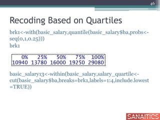
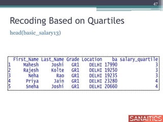
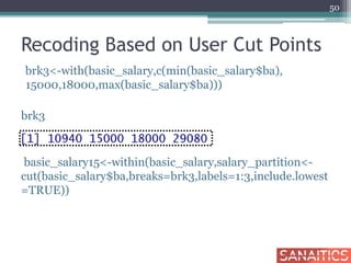
51. Recoding Based on User Cut Points
basic_salary15[c(20,30),]
51

52. Remove Variables
#using remove.vars function (need to load “gdata”
package)
Removing variable 'Name'
Removing variable 'Place‘
basic_salary<-remove.vars(basic_salary,c("Last_Name",
"Location"))
names(basic_salary)
[1] "X" "First_Name" "Grade" "ba"
52

53. Sorting & Merging
53

54. Sorting Data
attach(basic_salary)
bs_sorted1<-basic_salary[order(-ba), ]
head(bs_sorted1)
54

55. Sorting by Multiple Variables
bs_sorted2<-basic_salary[order( First_Name, ba) , ]
head(bs_sorted2)
55

56. Merging by Variables
Create the below two datasets
sal_data
bonus_data
56

57. Outer Join
outerjoin<-
merge(sal_data,bonus_data,by=c("Employee_ID"),all=
TRUE)
outerjoin
57

58. Inner Join
innerjoin<-
merge(sal_data,bonus_data,by=("Employee_ID"))
innerjoin
58

59. Left Join
leftjoin<-merge(sal_data,bonus_data,
by=c("Employee_ID"),all.x=TRUE)
leftjoin
59

60. Right Join
right_join<-merge(sal_data,bonus_data,
by="Employee_ID" , all.y=TRUE)
right_join
60

61. Merging Cases (append)
# rbind function
Appending two datasets using rbind function requires
both the datasets with exactly the same number of
variables with exactly the same names
If datasets do not have the same number of variables ,
variables can be either dropped or created so both
match.
or else
# smartbind function can be used
#need to donwload gtools package to use this function
61

62. R-String Functions
basic_salary$Location<-substr(basic_salary$Location,1,1)
head(basic_salary)
62

63. Replace Function
basic_salary$Location<-substr(basic_salary$Location,1,1)
head(basic_salary)
table(basic_salary$Location)
63

64. Contd…..
replace Function
replace() function replaces the values in x with indices given in list by those
given in values. If necessary, the values in values are recycled.
64

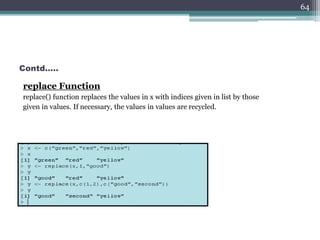
65. Deleting missing cases# complete.cases, na.exclude(), na.omit()are for dealing manually with NAs in a
dataset
x<-c(12,NA,13,12)
y<-c(25,48,NA,NA)
data<-data.frame(x,y)
data
65
data1<-na.omit(data)
data1
x y
1 12 25
data[complete.cases(da
ta),]
x y
1 12 25
na.exclude(data)
x y
1 12 25

66. Thank you !!!!
66