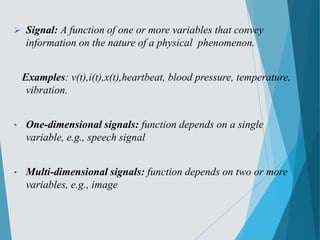
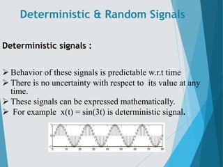
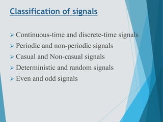
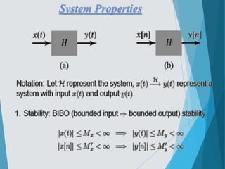
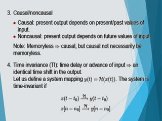
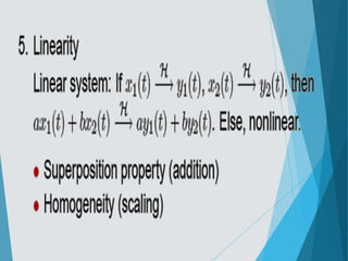
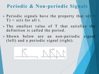
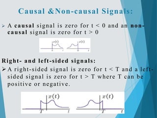
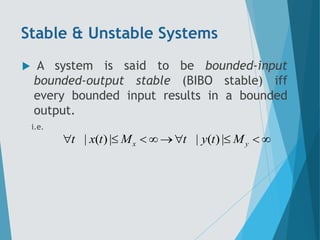
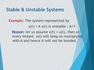
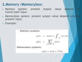
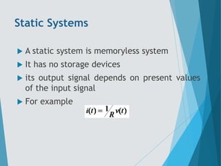
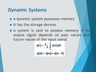
This document provides an overview of signals and systems classification. It discusses: 1) Signals can be continuous-time or discrete-time, periodic or non-periodic, deterministic or random, even or odd. 2) Systems can be causal or non-causal, linear or nonlinear, time-invariant or time-variant, stable or unstable. 3) Key system properties include memory/memoryless, and examples of discrete-time systems are presented.

1. Department of Electronics & Communication Engineering
Presentation
On
Classification of Signals & Systems
Guided by:-
Sanjeet K Shriwastava
Asst . Prof(ECE)
LIT, Sarigam.
Submitted by:-
Name: Enrollnment No.
Jay Baria 150860111003
Laxmi Institute of Technology, Sarigam
Approved by AICTE, New Delhi; Affiliated to Gujarat Technological University,
Ahmedabad

2.  Signals are variables that carry information.
 It is described as a function of one or more
independent variables.
 Basically it is a physical quantity.It varies with
some independent or dependent variables.
 Signals can be One-dimensional or multi-
dimensional.
Introduction to Signals

3.  Signal: A function of one or more variables that convey
information on the nature of a physical phenomenon.
Examples: v(t),i(t),x(t),heartbeat, blood pressure, temperature,
vibration.
• One-dimensional signals: function depends on a single
variable, e.g., speech signal
• Multi-dimensional signals: function depends on two or more
variables, e.g., image

4. Classification of signals
 Continuous-time and discrete-time signals
 Periodic and non-periodic signals
 Casual and Non-casual signals
 Deterministic and random signals
 Even and odd signals

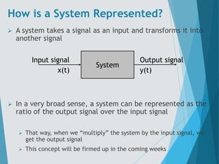
5. Continuous time (CT) &
discrete time (DT) signals:
 CT signals take on real or complex values as a
function of an independent variable that ranges over
the real numbers and are denoted as x(t).
 DT signals take on real or complex values as a
function of an independent variable that ranges over
the integers and are denoted as x[n].
 Note the subtle use of parentheses and square
brackets to distinguish between CT and DT signals.

6. Periodic & Non-periodic Signals
 Periodic signals have the property that x(t +
T) = x(t) for all t.
 The smallest value of T that satisfies the
definition is called the period.
 Shown below are an non-periodic signal
(left) and a periodic signal (right).

7.  A causal signal is zero for t < 0 and an non-
causal signal is zero for t > 0
Right- and left-sided signals:
 A right-sided signal is zero for t < T and a left -
sided signal is zero for t > T where T can be
positive or negative.
Causal &Non-causal Signals:

8. Deterministic & Random Signals
Deterministic signals :
 Behavior of these signals is predictable w.r.t time
 There is no uncertainty with respect to its value at any
time.
 These signals can be expressed mathematically.
 For example x(t) = sin(3t) is deterministic signal.

9.  Behavior of these signals is random i.e. not predictable
w.r.t time.
 There is an uncertainty with respect to its value at any
time.
 These signals can’t be expressed mathematically.
 For example:Thermal Noise generated is non deterministic
signal.
Random Signals:

10. Even &Odd Signals
 Even signals xe(t) and odd signals xo(t) are defined
as
xe (t) = xe (−t) and xo (t) = −xo (−t).
 Any signal is a sum of unique odd and even signals.
Using
x(t) = xe(t)+xo(t) and x(−t) = xe(t) − xo(t), yields
xe(t) =0.5(x(t)+x(−t)) and xo(t) =0.5(x(t) − x(−t)).

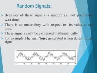
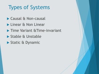
11. Even:
x(−t) = x(t)
x[−n] = x[n]
Odd:
x(−t) = −x(t)
x[−n] = −x[n]
 Any signal x(t) can be expressed as
x(t) = xe(t) + xo(t) )
x(−t) = xe(t) − xo(t)
where
xe(t) = 1/2(x(t) + x(−t))
xo(t) = 1/2(x(t) − x(−t))
Even &Odd Signals:

12. Bounded &Unbounded Signals:
 Every system is bounded, but meaningful
signal is always bounded

13. Power and Energy Signals
 Power Signal
 Infinite duration
 Normalized power is
finite and non-zero
 Normalized energy
averaged over infinite
time is infinite
 Mathematically
tractable
 Energy Signal
 Finite duration
 Normalized energy is
finite and non-zero
 Normalized power
averaged over infinite
time is zero
 Physically realizable

14. Elementary signals
 Step function
 Impulse function
 Ramp function

15. Unit Step function:

16. Unit ramp function:
Unit impulse function:

17. What is a System?
 Systems process input signals to produce output signals.
 Examples:
 A circuit involving a capacitor can be viewed as a system that
transforms the source voltage (signal) to the voltage (signal)
across the capacitor
 A CD player takes the signal on the CD and transforms it into a
signal sent to the loud speaker
 A communication system is generally composed of three sub-
systems, the transmitter, the channel and the receiver. The
channel typically attenuates and adds noise to the transmitted
signal which must be processed by the receiver

18. How is a System Represented?
 A system takes a signal as an input and transforms it into
another signal
 In a very broad sense, a system can be represented as the
ratio of the output signal over the input signal
 That way, when we “multiply” the system by the input signal, we
get the output signal
 This concept will be firmed up in the coming weeks
System
Input signal
x(t)
Output signal
y(t)

19. Types of Systems
 Causal & Non-causal
 Linear & Non Linear
 Time Variant &Time-invariant
 Stable & Unstable
 Static & Dynamic

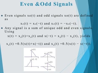
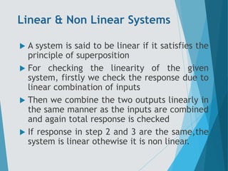
20. Causal Systems
 Causal system : A system is said to be causal
if the present value of the output signal
depends only on the present and/or past
values of the input signal.
 Example: y[n]=x[n]+1/2x[n-1]

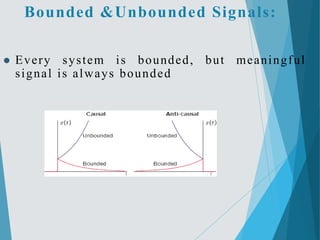
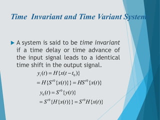
21. Non-causal Systems
 Non-causal system : A system is said to be
anticausal if the present value of the output signal
depends only on the future values of the input
signal.
 Example: y[n]=x[n+1]+1/2x[n-1]

22. Linear & Non Linear Systems
 A system is said to be linear if it satisfies the
principle of superposition
 For checking the linearity of the given
system, firstly we check the response due to
linear combination of inputs
 Then we combine the two outputs linearly in
the same manner as the inputs are combined
and again total response is checked
 If response in step 2 and 3 are the same,the
system is linear othewise it is non linear.

23. Time Invariant and Time Variant Systems
 A system is said to be time invariant
if a time delay or time advance of
the input signal leads to a identical
time shift in the output signal.
0
0 0
( ) { ( )}
{ { ( )}} { ( )}
i
t t
y t H x t t
H S x t HS x t
 
 
0
0
0 0
( ) { ( )}
{ { ( )}} { ( )}
t
t t
y t S y t
S H x t S H x t

 

24. Linear Time-Invariant Systems
 Special importance for their mathematical tractability
 Most signal processing applications involve LTI systems
 LTI system can be completely characterized by their
impulse response
       
   
     
[ ]
k
k
k k
y n T x n T x k n k Linearity
x k T n k x k h n Time Inv




 
 
 
  
 
 
  

 
       
k
x k h n k x k h k


  


25. Stable & Unstable Systems
 A system is said to be bounded-input
bounded-output stable (BIBO stable) iff
every bounded input results in a bounded
output.
i.e.
| ( )| | ( )|
x y
t x t M t y t M
       

26. Stable & Unstable Systems
Example: The system represented by
y(t) = A x(t) is unstable ; A˃1
Reason: let us assume x(t) = u(t), then at
every instant u(t) will keep on multiplying
with A and hence it will not be bonded.

27. Static Systems
 A static system is memoryless system
 It has no storage devices
 its output signal depends on present values
of the input signal
 For example

28. Dynamic Systems
 A dynamic system possesses memory
 It has the storage devices
 A system is said to possess memory if its
output signal depends on past values and
future values of the input signal

29. Memoryless System
A system is memoryless if the output y[n] at every value
of n depends only on the input x[n] at the same value of n
Example :
Square
Sign
counter example:
Ideal Delay System
 2
]
n
[
x
]
n
[
y 
 
]
n
[
x
sign
]
n
[
y 
]
n
n
[
x
]
n
[
y o



30. Discrete-Time Systems
 Discrete-Time Sequence is a mathematical operation that maps a
given input sequence x[n] into an output sequence y[n]
 Example Discrete-Time Systems
 Moving (Running) Average
 Maximum
 Ideal Delay System
]}
n
[
x
{
T
]
n
[
y  T{.}
x[n] y[n]
]
3
n
[
x
]
2
n
[
x
]
1
n
[
x
]
n
[
x
]
n
[
y 






 
]
2
n
[
x
],
1
n
[
x
],
n
[
x
max
]
n
[
y 


]
n
n
[
x
]
n
[
y o



31. System Properties

32. 2.Memory /Memoryless:
 Memory system: present output value depend on
future/past input.
 Memoryless system: present output value depend only on
present input.
 Example:

35. Properties of a System:
 On this course, we shall be particularly interested in signals with
certain properties:
 Causal: a system is causal if the output at a time, only depends on
input values up to that time.
 Linear: a system is linear if the output of the scaled sum of two
input signals is the equivalent scaled sum of outputs
 Time-invariance: a system is time invariant if the system’s
output is the same, given the same input signal, regardless of
time.
 These properties define a large class of tractable, useful systems
and will be further considered in the coming lectures