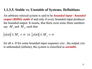
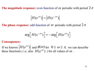
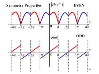
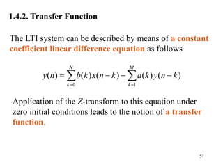
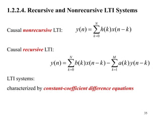
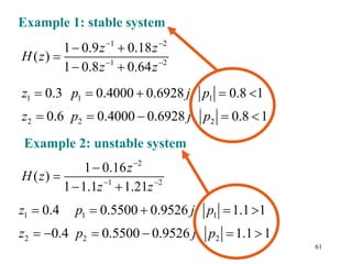
1. The document summarizes a lecture on discrete-time signals and systems. 2. It defines different types of signals, including discrete-time and discrete-valued signals which are relevant for digital filter theory. 3. It also classifies systems as static vs. dynamic, time-invariant vs. time-variable, linear vs. nonlinear, causal vs. non-causal, stable vs. unstable, and recursive vs. non-recursive. 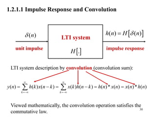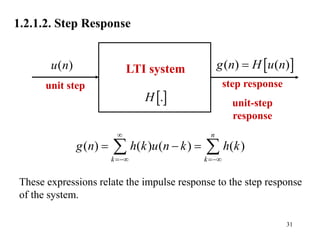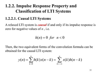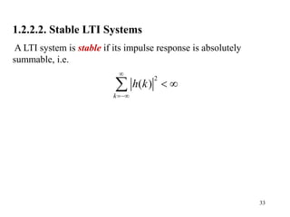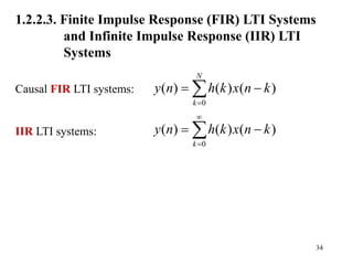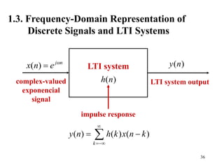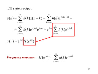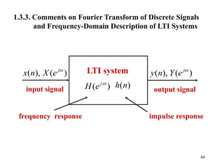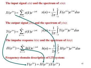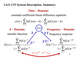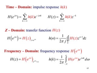4. It describes the time-domain representation of linear, time-invariant (LTI) systems using impulse response and convolution.

1. 1
Lecture 1: February 20, 2007
Topic:
1. Discrete-Time Signals and Systems

2. 2
Lecture 1: February 20, 2007
Topic:
1. Discrete-Time Signals and Systems
• signal classification -> signals to be applied in digital filter
theory within our course,
• some elementary discrete-time signals,
• discrete-time systems: definition, basic properties review,
discrete-time system classification, input-output model of
discrete-time systems -> system to be applied in digital filter
theory within our course,
• Linear discrete-time time-invariant system description in
time-, frequency- and transform-domain.

3. 3
1. Discrete-Time Signals and
Systems. Summary
1.1. Basic Definitions

4. 4
1.1.1. Discrete and Digital Signals
1.1.1.1. Basic Definitions
Signals may be classified into four categories depending
on the characteristics of the time-variable and values
they can take:
• continuous-time signals (analogue signals),
• discrete-time signals,
• continuous-valued signals,
• discrete-valued signals.

5. 5
Continuous-time (analogue) signals:
Time: defined for every value of time ,
Descriptions: functions of a continuous variable t: ,
Notes: they take on values in the continuous
interval .
( )
f t
( ) ( , ) ,
f t a b for a b
   
t R

Note: ( )
( )
( , ) ( , )
,
f t C
f t j
a b and a b
a b
 
 

 
   
 

6. 6
Discrete-time signals:
Time: defined only at discrete values of time: ,
Descriptions: sequences of real or complex
numbers ,
Note A.: they take on values in the continuous
interval ,
Note B.: sampling of analogue signals:
• sampling interval, period: ,
• sampling rate: number of samples per
second,
• sampling frequency (Hz): .
( ) ( )
f nT f n

T
1/
S
f T

( ) ( , ) ,
f n a b for a b
   
t nT


7. 7
Continuous-valued signals:
Time: they are defined for every value of time or
only at discrete values of time,
Value: they can take on all possible values on
finite or infinite range,
Descriptions: functions of a continuous variable
or sequences of numbers.

8. 8
Discrete-valued signals:
Time: they are defined for every value of time or
only at discrete values of time,
Value: they can take on values from a finite set of
possible values,
Descriptions: functions of a continuous variable or
sequences of numbers.

9. 9
Digital filter theory:
Digital signals:
Definition and descriptions: discrete-time and
discrete-valued signals (i.e. discrete -time
signals taking on values from a finite set of
possible values),
Note: sampling, quatizing and coding process i.e.
process of analogue-to-digital conversion.
Discrete-time signals:
Definition and descriptions: defined only at discrete
values of time and they can take all possible
values on finite or infinite range (sequences of
real or complex numbers: ),
Note: sampling process, constant sampling period.
( )
f n

10. 10
1.1.1.2. Discrete-Time Signal Representations
A. Functional representation:
1 1,3
( ) 6 0,7
0
for n
x n for n
elsewhere



 



0 0
( ) 0,6 0,1, ,102
1 102
n
for n
y n for n
n



 

 

B. Graphical
representation
( )
x n
n

11. 11
D. Sequence representation:
 
( ) 0.12 2.01 1.78 5.23 0.12
x n 
n … -2 -1 0 1 2
x(n) … 0.12 2.01 1.78 5.23 0.12
C. Tabular representation:

12. 12
1.1.1.3. Elementary Discrete-Time Signals
A. Unit sample sequence (unit sample, unit impulse,
unit impulse signal)
1 0
( )
0 0
for n
n
for n



 


( )
n

n

13. 13
B. Unit step signal (unit step, Heaviside step sequence)
1 0
( )
0 0
for n
u n
for n


 


n
( )
u n

14. 14
C. Complex-valued exponential signal
 
2 .
( ) , ( ) 1, arg ( ) 2 .
j nT
S
f n
x n e x n x n nT f nT
f
 
 
    
where
, , 1
R n N j is imaginary unit
    
and
T is sampling period and is sampling frequency.
S
f
(complex sinusoidal sequence, complex phasor)

15. 15
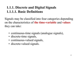
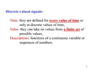
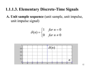
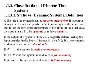
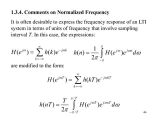
1.1.2. Discrete-Time Systems. Definition
A discrete-time system is a device or algorithm that
operates on a discrete-time signal called the input or
excitation (e.g. x(n)), according to some rule (e.g. H[.])
to produce another discrete-time signal called the output
or response (e.g. y(n)).
 
( ) ( )
y n H x n

This expression denotes also the transformation H[.]
(also called operator or mapping) or processing
performed by the system on x(n) to produce y(n).

16. 16
( )
x n
input signal
excitation
( )
y n
output signal
response
( ) ( )
H
x n y n


 
( ) ( )
y n H x n


.
H
discrete-time
system
Input-Output Model of Discrete-Time System
(input-output relationship description)

17. 17
1.1.3. Classification of Discrete-Time
Systems
1.1.3.1. Static vs. Dynamic Systems. Definition
A discrete-time system is called static or memoryless if its output
at any time instant n depends on the input sample at the same time,
but not on the past or future samples of the input. In the other case,
the system is said to be dynamic or to have memory.
If the output of a system at time n is completly determined by the
input samples in the interval from n-N to n ( ), the system is
said to have memory of duration N.
If , the system is static or memoryless.
If , the system is said to have finite memory.
If , the system is said to have infinite memory.
0
N 
0
N 
0 N
  
N  

18. 18
Examples:
The static (memoryless) systems:
The dynamic systems with finite memory:
The dynamic system with infinite memory:
3
( ) ( ) ( )
y n nx n bx n
 
0
( ) ( ) ( )
N
k
y n h k x n k

 

0
( ) ( ) ( )
k
y n h k x n k


 


19. 19
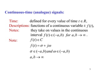
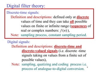
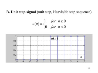
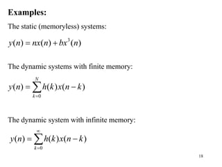
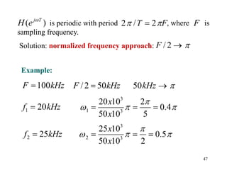
1.1.3.2. Time-Invariant vs. Time-Variable Systems.
Definition
A discrete-time system is called time-invariant if its input-output
characteristics do not change with time. In the other case, the
system is called time-variable.
Definition. A relaxed system is time- or shift-invariant if
only if
implies that
for every input signal and every time shift k .
[.]
H
( ) ( )
H
x n y n


( ) ( )
H
x n k y n k
 
 
( )
x n
 
( ) ( )
y n H x n

 
( ) ( )
y n k H x n k
  

20. 20
Examples:
The time-invariant systems:
The time-variable systems:
3
( ) ( ) ( )
y n x n bx n
 
0
( ) ( ) ( )
N
k
y n h k x n k

 

3
( ) ( ) ( 1)
y n nx n bx n
  
0
( ) ( ) ( )
N
N n
k
y n h k x n k


 


21. 21
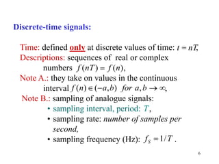
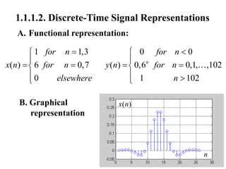
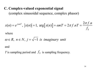
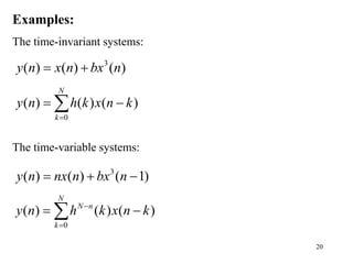
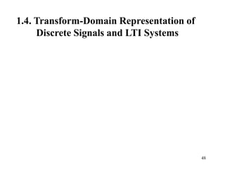
1.1.3.3. Linear vs. Non-linear Systems. Definition
A discrete-time system is called linear if only if it satisfies the linear
superposition principle. In the other case, the system is called non-
linear.
Definition. A relaxed system is linear if only if
for any arbitrary input sequences and , and any
arbitrary constants and .
The multiplicative (scaling) property of a linear system:
The additivity property of a linear system:
[.]
H
     
1 1 2 2 1 1 2 2
( ) ( ) ( ) ( )
H a x n a x n a H x n a H x n
  
1( )
x n 2 ( )
x n
1
a 2
a
   
1 1 1 1
( ) ( )
H a x n a H x n

     
1 2 1 2
( ) ( ) ( ) ( )
H x n x n H x n H x n
  

22. 22
Examples:
The linear systems:
The non-linear systems:
0
( ) ( ) ( )
N
k
y n h k x n k

 
 2
( ) ( ) ( )
y n x n bx n k
  
3
( ) ( ) ( 1)
y n nx n bx n
  
0
( ) ( ) ( ) ( 1)
N
k
y n h k x n k x n k

   


23. 23
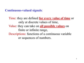
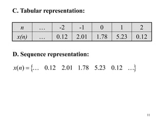
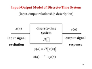
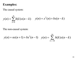
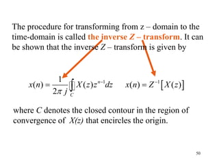
1.1.3.4. Causal vs. Non-causal Systems. Definition
Definition. A system is said to be causal if the output of the system
at any time n (i.e., y(n)) depends only on present and past inputs
(i.e., x(n), x(n-1), x(n-2), … ). In mathematical terms, the output of a
causal system satisfies an equation of the form
where is some arbitrary function. If a system does not satisfy
this definition, it is called non-causal.
 
( ) ( ), ( 1), ( 2),
y n F x n x n x n
  
[.]
F

24. 24
Examples:
The causal system:
The non-causal system:
0
( ) ( ) ( )
N
k
y n h k x n k

 

2
( ) ( ) ( )
y n x n bx n k
  
3
( ) ( 1) ( 1)
y n nx n bx n
   
10
10
( ) ( ) ( )
k
y n h k x n k

 


25. 25
1.1.3.5. Stable vs. Unstable of Systems. Definitions
An arbitrary relaxed system is said to be bounded input - bounded
output (BIBO) stable if and only if every bounded input produces
the bounded output. It means, that there exist some finite numbers
say and , such that
for all n. If for some bounded input sequence x(n) , the output y(n)
is unbounded (infinite), the system is classified as unstable.
x
M y
M
( ) ( )
x y
x n M y n M
      

26. 26
Examples:
The stable systems:
The unstable system:
0
( ) ( ) ( )
N
k
y n h k x n k

 

2
( ) ( ) 3 ( )
y n x n x n k
  
3
( ) 3 ( 1)
n
y n x n
 

27. 27
1.1.3.6. Recursive vs. Non-recursive Systems.
Definitions
A system whose output y(n) at time n depends on any number of the
past outputs values ( e.g. y(n-1), y(n-2), … ), is called a recursive
system. Then, the output of a causal recursive system can be
expressed in general as
where F[.] is some arbitrary function. In contrast, if y(n) at time n
depends only on the present and past inputs
then such a system is called nonrecursive.
 
( ) ( 1), ( 2), , ( ), ( ), ( 1), , ( )
y n F y n y n y n N x n x n x n M
     
 
( ) ( ), ( 1), , ( )
y n F x n x n x n M
  

28. 28
Examples:
The nonrecursive system:
The recursive system:
0
( ) ( ) ( )
N
k
y n h k x n k

 

0 1
( ) ( ) ( ) ( ) ( )
N N
k k
y n b k x n k a k y n k
 
   
 

29. 29
1.2. Linear-Discrete Time Time-Invariant
Systems (LTI Systems)
1.2.1. Time-Domain Representation

30. 30

.
H
LTI system
unit impulse
( )
n
  
( ) ( )
h n H n


impulse response
LTI system description by convolution (convolution sum):
Viewed mathematically, the convolution operation satisfies the
commutative law.
( ) ( ) ( ) ( ) ( ) ( )* ( ) ( )* ( )
k k
y n h k x n k x k h n k h n x n x n h n
 
 
     
 
1.2.1.1 Impulse Response and Convolution

31. 31
1.2.1.2. Step Response

.
H
unit step
( )
u n
step response
unit-step
response
 
( ) ( )
g n H u n

( ) ( ) ( ) ( )
n
k k
g n h k u n k h k

 
  
 
These expressions relate the impulse response to the step response
of the system.
LTI system

32. 32
1.2.2. Impulse Response Property and
Classification of LTI Systems
1.2.2.1. Causal LTI Systems
A relaxed LTI system is causal if and only if its impulse response is
zero for negative values of n , i.e.
Then, the two equivalent forms of the convolution formula can be
obtained for the causal LTI system:
( ) 0 0
h n for n
 
0
( ) ( ) ( ) ( ) ( )
n
k k
y n h k x n k x k h n k

 
   
 

33. 33
1.2.2.2. Stable LTI Systems
A LTI system is stable if its impulse response is absolutely
summable, i.e.
2
( )
k
h k


 


34. 34
1.2.2.3. Finite Impulse Response (FIR) LTI Systems
and Infinite Impulse Response (IIR) LTI
Systems
Causal FIR LTI systems:
IIR LTI systems:
0
( ) ( ) ( )
N
k
y n h k x n k

 

0
( ) ( ) ( )
k
y n h k x n k


 


35. 35
1.2.2.4. Recursive and Nonrecursive LTI Systems
Causal nonrecursive LTI:
Causal recursive LTI:
LTI systems:
characterized by constant-coefficient difference equations
0
( ) ( ) ( )
N
k
y n h k x n k

 

0 1
( ) ( ) ( ) ( ) ( )
N M
k k
y n b k x n k a k y n k
 
   
 

36. 36
1.3. Frequency-Domain Representation of
Discrete Signals and LTI Systems
LTI system
( )
h n
complex-valued
exponencial
signal
( ) j n
x n e 

impulse response
( ) ( ) ( )
k
y n h k x n k


 

LTI system output
( )
y n

37. 37
LTI system output:
( )
( ) ( ) ( ) ( )
( ) ( )
j n k
k k
j k j n j n j k
k k
y n h k x n k h k e
h k e e e h k e

   
 

 
 
 
 
   
 
 
 
( ) ( )
j n j
y n e H e
 

Frequency response: ( ) ( )
j j k
k
H e h k e
 



 

38. 38
( )
( ) ( )
j j j
H e H e e
   

( ) Re ( ) Im ( )
j j j
H e H e j H e
  
   
 
   
( ) ( )cos ( )sin
j
k k
H e h k k j h k k

 
 
 
 
  
 
 
 
Re ( ) ( )cos
j
k
H e h k k




  
  
Im ( ) ( )sin
j
k
H e h k k




   
  

39. 39
Magnitude response:
2 2
( ) Re ( ) Im ( )
j j j
H e H e H e
  
   
 
   
Im ( )
( ) arg ( )
Re ( )
j
j
j
H e
H e arctg
H e



 
 
 
 
 
   
 
Phase response:
( )
( )
d
d
 
 

 
Group delay function:

40. 40
1.3.1. Comments on relationship between the impulse
response and frequency response
The important property of the frequency response
is fact that this function is periodic with period .
2
   
2 2
( ) ( ) ( ) ( )
j l j l
j j k
k k
H e h k e h k e H e
   
 
 
  

 
  
 
( )
j
H e 
( )
j
H e 
1
( ) ( )
2
j j n
h n H e e d

 


 
 
In fact, we may view the previous expression as the exponential
Fourier series expansion for , with h(k) as the Fourier series
coefficients. Consequently, the unit impulse response h(k) is related
to through the integral expression

41. 41
1.3.2. Comments on symmetry properties
For LTI systems with real-valued impulse response, the magnitude
response, phase responses, the real component of and the imaginary
component of possess these symmetry properties:
The real component: even function of periodic with period
The imaginary component: odd function of periodic with period
( )
j
H e 


2
2
Re ( ) Re ( )
j j
H e H e
 

   

   
Im ( ) Im ( )
j j
H e H e
 

   
 
   

42. 42
The magnitude response: even function of periodic with period
The phase response: odd function of periodic with period
 2
( ) ( )
j j
H e H e
 


 2
arg ( ) arg ( )
j j
H e H e
 

   
 
   
Consequence:
If we known and for , we can describe
these functions ( i.e. also ) for all values of .
( )
j
H e 
( )
  0  
 
( )
j
H e 


43. 43
( )
j
H e 

 2


4
 3
 2
 3 4

 2


4
 3
 2
 3 4
Symmetry Properties
( )
 
EVEN
ODD
0
0

44. 44
1.3.3. Comments on Fourier Transform of Discrete Signals
and Frequency-Domain Description of LTI Systems
LTI system
( )
h n
impulse response
( )
j
H e 
frequency response
input signal
( ), ( )
j
x n X e 
output signal
( ), ( )
j
y n Y e 

45. 45
The input signal x(n) and the spectrum of x(n):
( ) ( )
j j k
k
X e x k e
 



 
1
( ) ( )
2
j j n
x n X e e d

 


 
 
( ) ( )
j j k
k
Y e y k e
 



 
1
( ) ( )
2
j j n
y n Y e e d

 


 
 
The output signal y(n) and the spectrum of y(n):
( ) ( )
j j k
k
H e h k e
 



 
1
( ) ( )
2
j j n
h n H e e d

 


 
 
The impulse response h(n) and the spectrum of h(n):
Frequency-domain description of LTI system:
( ) ( ) ( )
j j j
Y e H e X e
  


46. 46
1.3.4. Comments on Normalized Frequency
It is often desirable to express the frequency response of an LTI
system in terms of units of frequency that involve sampling
interval T. In this case, the expressions:
( ) ( )
j j k
k
H e h k e
 



 
1
( ) ( )
2
j j n
h n H e e d

 


 
 
are modified to the form:
( ) ( )
j T j kT
k
H e h kT e
 



 
/
/
( ) ( )
2
T
j T j nT
T
T
h nT H e e d

 


 
 

47. 47
is periodic with period , where is
sampling frequency.
Solution: normalized frequency approach:
( )
j T
H e 
2 / 2
T F
 
 F
/2
F 

/2 50
F kHz
 50kHz 

3
1 3
20 10 2
0.4
50 10 5
x
x

  
  
3
2 3
25 10
0.5
50 10 2
x
x

  
  
100
F kHz

1 20
f kHz

2 25
f kHz

Example:

48. 48
1.4. Transform-Domain Representation of
Discrete Signals and LTI Systems

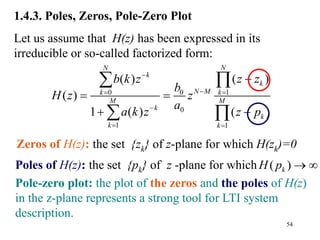
49. 49
1.4.1. Z -Transform
Since Z – transform is an infinite power series, it exists
only for those values of z for which this series converges.
The region of convergence of X(z) is the set of all values
of z for which X(z) attains a finite value.
Definition: The Z – transform of a discrete-time signal x(n)
is defined as the power series:
( ) ( ) k
k
X z x n z



  ( ) [ ( )]
X z Z x n

where z is a complex variable. The above given relations
are sometimes called the direct Z - transform because
they transform the time-domain signal x(n) into its
complex-plane representation X(z).

50. 50
The procedure for transforming from z – domain to the
time-domain is called the inverse Z – transform. It can
be shown that the inverse Z – transform is given by
1
1
( ) ( )
2
n
C
x n X z z dz
j


   
1
( ) ( )
x n Z X z


where C denotes the closed contour in the region of
convergence of X(z) that encircles the origin.

51. 51
1.4.2. Transfer Function
0 1
( ) ( ) ( ) ( ) ( )
N M
k k
y n b k x n k a k y n k
 
   
 
Application of the Z-transform to this equation under
zero initial conditions leads to the notion of a transfer
function.
The LTI system can be described by means of a constant
coefficient linear difference equation as follows

52. 52
LTI System
 
( ) ( )
Y z Z y n

input signal
( )
x n
 
( ) ( )
X z Z x n

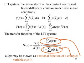
Transfer function: the ratio of the Z - transform of the
output signal and the Z - transform of the input signal of
the LTI system:
( ) [ ( )]
( )
( ) [ ( )]
Y z Z y n
H z
X z Z x n
 
output signal
( )
y n
( )
H z
 
( ) ( )
H z Z h n

( )
h n

53. 53
LTI system: the Z-transform of the constant coefficient
linear difference equation under zero initial
conditions:
0 1
( ) ( ) ( ) ( ) ( )
N M
k k
k k
Y z b k z X z a k z Y z
 
 
 
 
The transfer function of the LTI system:
0
1
( )
( )
( )
( )
1 ( )
N
k
k
M
k
k
b k z
Y z
H z
X z
a k z




 



0 1
( ) ( ) ( ) ( ) ( )
N M
k k
y n b k x n k a k y n k
 
   
 
H(z): may be viewed as a rational function of a complex
variable z (z-1).

54. 54
1.4.3. Poles, Zeros, Pole-Zero Plot
Let us assume that H(z) has been expressed in its
irreducible or so-called factorized form:
0
0 1
0
1 1
( )
( )
( )
1 ( ) ( )
N
N
k
k
N M
k k
M M
k
k
k k
z z
b k z
b
H z z
a
a k z z p


 

 

 
 
 
 
Pole-zero plot: the plot of the zeros and the poles of H(z)
in the z-plane represents a strong tool for LTI system
description.
Zeros of H(z): the set {zk} of z-plane for which H(zk)=0
Poles of H(z): the set {pk} of z -plane for which ( )
k
H p  

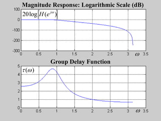
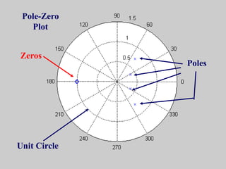
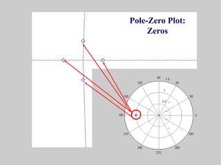
55. 55
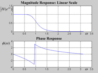
Example: the 4-th order Butterworth low-pass filter,
cut off frequency .
1 3

 
0
1
( )
( )
1 ( )
N
k
k
M
k
k
b k z
H z
a k z








z1= -1.0002, z2= -1.0000 + 0.0002j
z3= -1.0000 - 0.0002j, z4= -0.9998
0
1
( )
( )
1 ( )
N
k
k
M
k
k
b k z
H z
a k z








b =[ 0.0186 0.0743 0.1114 0.0743 0.0186 ]
a =[ 1.0000 -1.5704 1.2756 -0.4844 0.0762 ]
p1= 0.4488 + 0.5707j, p2= 0.4488 - 0.5707j
p3= 0.3364 + 0.1772j, p4= 0.3364 - 0.1772j

56. 56
Magnitude Response: Linear Scale
Phase Response
( )
j
H e 
( )
 



57. 57
Magnitude Response: Logarithmic Scale (dB)
Group Delay Function
20log ( )
j
H e 


( )
 

58. 58
Pole-Zero
Plot
Unit Circle
Poles
Zeros

59. 59
Pole-Zero Plot:
Zeros

60. 60
1.4.4. Transfer Function and Stability of LTI Systems
Condition: LTI system is BIBO stable if and only if the
unit circle falls within the region of convergence of the
power series expansion for its transfer function. In the
case when the transfer function characterizes a causal LTI
system, the stability condition is equivalent to the
requirement that the transfer function H(z) has all of its
poles inside the unit circle.

61. 61
Example 1: stable system
Example 2: unstable system
2
1 2
1 0.16
( )
1 1.1 1.21
z
H z
z z

 


 
1 1 1
2 2 2
0.4 0.5500 0.9526 1.1 1
0.4 0.5500 0.9526 1.1 1
z p j p
z p j p
    
     
1 2
1 2
1 0.9 0.18
( )
1 0.8 0.64
z z
H z
z z
 
 
 

 
1 1 1
2 2 2
0.3 0.4000 0.6928 0.8 1
0.6 0.4000 0.6928 0.8 1
z p j p
z p j p
    
    

62. 62
Z – Domain:
0
1
( )
( )
1 ( )
N
k
k
M
k
k
b k z
H z
a k z








transfer function
Frequency – Domain:
0
1
( )
( )
1 ( )
N
j k
j k
M
j k
k
b k e
H e
a k e











frequency response
Time – Domain:
0 1
( ) ( ) ( ) ( ) ( )
N M
k k
y n b k x n k a k y n k
 
   
 
constant coefficient linear difference equation
1.4.5. LTI System Description. Summary
j j
z e e z
 
 
h(n)
Z
Z-1 FT-1
FT

63. 63
( )
H z
Z – Domain: transfer function
    jw
j
z e
H z
H e 

 1
1
)
( ) (
2
n
C
H z
h n z dz
j


 
( )
h k
Time – Domain: impulse response
( ) ( )
j j k
k
H e e
h k
 



  )
( (
) k
k
H z z
h k



 
Frequency – Domain: frequency response
 
( ) j
j
e z
e
H z H 


 (
2
)
) (
1 j k
j
H d
e
h k e





 
 
 
j
H e 