Lecture: Digital Signal Processing Batch 2009

Digital Signal Processing
Instructor:
Engr. Abdul Rauf Khan
Rajput

Engr. A. R.K. Rajput NFC IET 1
Multan

Books.

Text Books:
Principles, Algorithms and Applications
By:
John G.Proakis & Dimitris G.Manolakis
Reference Books
1. Digital Signal Processing By.
Sen M. Kuo & Woon-Seng Gan
2. Digital Signal Processing A Practical Approach. By
Emmanuel C. Ifeachor & Barrie W. Jervis
[Handouts]
Digital Signal Processing By. Bores [Avail at ww.bores.com/courses/
Multan

Grading Policy

Term Papers/test/Group Discussion 20 Marks
Mid-Term 30 Marks
Final 50 Marks

Additional Privileges 10%
Trem Paper. Home works, Presentations, Voluntary
assignments managements etc.

Class will be divided different level as per their GPA
Group A- GPA 2.0 to 2.59
Group B- GPA 2.5 to 3.39
Group C – GPA 3.4 to 4
Multan

Signal : f(x1: x2……….. ) is function, A function is a dependent variable of independent
variable(s).
X= Time, Distance, Temperature,….
Type of signal Natural Signal [1D,2D,MD]
Continuous? Discrete Signal
Analog Signal = 1-Cont-time--- 2-Discrete Time ---- A/D -----Digital Signal

Analog and Digital Signals
Analog signal = continuous-time + continuous amplitude

Digital signal = discrete-time + discrete amplitude

Signal Processing
analog system = analog signal input + analog signal output
advantages: easy to interface to real world, do not need A/D or D/A converters,
speed not dependent on clock rate
digital system = digital signal input + digital signal output I re-configurability
using software, greater control over accuracy/resolution, predictable and reproducible A.S
behavior D.S M.
Engr. A. R.K. Rajput NFC IET Multan
.p .p
4
S.p

Analog-to-Digital Conversion

0101...
Sampler X(n)
Discrete-
Quantize r xq(t) Coder Digital Signal
x(t)
Quantiz
time
ed
signal Signal

Sampling:
conversion from cts-time to dst-time by taking samples" at discrete time instants E.g.,
uniform sampling: x(n) = xa(nT) where T is the sampling period and n ε Z

Quantization: conversion from dst-time cts-valued signal to a dst-
time dst-valued signal quantization error: eq(n) = xq(n)- x(n))
Coding: representation of each dst-value xq(n) by a b-bit binary sequence

Multan

Sampling Theorem
If the highest frequency contained in an analog signal x a(t) is Fmax = B and the signal is
sampled at a rate
Fs > 2Fmax=2B
then xa(t) can be exactly recovered from its sample values using the interpolation
function Note: FN = 2B = 2Fmax
is called the Nyquist rate

Therefore, given the interpolation relation, x a(t) can be written as

where xa(nT) = x(n); called band limited interpolation.
Multan

Digital-to-Analog Conversion
Common interpolation approaches: bandlimited interpolation zero-order hold, linear interpolation,
higher-order interpolation techniques, e.g., using splines
In practice, cheap" interpolation along with a smoothing filter is employed.

A DSP System ????
Multan

A DSP System
In practice, a DSP system does not use idealized A/D or D/A
models.
Anti-aliasing Filter: ensures that analog input signal does not
contain frequency components higher than half of the
sampling frequency (to obey the sampling theorem). this
process is irreversible
2Sample and Hold:
holds a sampled analog value for a short time while the A/D
converts and interprets the value as a digital
3 A/D: converts a sampled data signal value into a digital
number, in part, through quantization of the amplitude
4 D/A: converts a digital signal into a staircase"-like signal
5 Reconstruction Filter: converts a staircase"-like signal
into an analog signal through low pass filtering similar to the
type used for anti-aliasing
Real-time DSP Considerations IET
Engr. A. R.K. Rajput NFC
Multan ??????? 8

Real-time DSP Considerations
What are initial considerations when designing a
DSP system that must run in real-time?

Is a DSP technology suitable for a real-time application?

Multan

Lecture 1
Week-1st

Multan

• Signal:
A signal is defined as a function of one or more variables
which conveys information on the nature of a physical
phenomenon. The value of the function can be a real
valued scalar quantity, a complex valued quantity, or
perhaps a vector.

• System:
A system is defined as an entity that manipulates one or
more signals to accomplish a function, thereby yielding
new signals.

Multan

• Continuos-Time Signal:
A signal x(t) is said to be a continuous time signal if it is
defined for all time t.

• Discrete-Time Signal:
A discrete time signal x[nT] has values specified only at
discrete points in time.
• Signal Processing:
A system characterized by the type of operation that it
performs on the signal. For example, if the operation is
linear, the system is called linear. If the operation is non-
linear, the system is said to be non-linear, and so forth.
Such operations are usually referred to as “Signal
Processing”.
Multan

Basic Elements of a Signal Processing
System
Analog input Analog output
signal Analog signal
Signal Processor

Analog Signal Processing

Analog Analog
input output
signal A/D Digital D/A signal
converter Signal Processor converter

Multan

• Advantages of Digital over Analogue Signal
Processing:
A digital programmable system allows flexibility in
reconfiguring the DSP operations simply by changing the
program. Reconfiguration of an analogue system usually
implies a redesign of hardware, testing and verification
that it operates properly.
DSP provides better control of accuracy requirements.

Digital signals are easily stored on magnetic media (tape
or disk).
The DSP allows for the implementation of more
sophisticated signal processing algorithms.
In some cases a digital implementation of the signal
processing system is cheaper than its analogue
counterpart. Engr. A. R.K. Rajput NFC IET 14
Multan

DSP Applications
Space photograph enhancement
Space Data compression
Intelligent sensory analysis
Diagnostic imaging (MRI, CT,
Medical ultrasound, etc.)
Electrocardiogram analysis
Medical image storage and retrieval

Image and sound compression for
Commercial multimedia presentation.
Movie special effects
Video conference calling

Video and data compression
Telephone echo reduction
signal multiplexing
filtering
Multan

DSP Applications (cont.)
Radar
Sonar
Military Ordnance Guidance
Secure communication
Oil and mineral prospecting
Industrial Process monitoring and control
Non-destructive testing

Earth quick recording and analysis
Data acquisition
Scientific Spectral Analysis
Simulation and Modeling

Multan

Classification of Signals

•Deterministic Signals
A deterministic signal behaves in a fixed known way with
respect to time. Thus, it can be modeled by a known
function of time t for continuous time signals, or a known
function of a sampler number n, and sampling spacing T
for discrete time signals.

• Random or Stochastic Signals:
In many practical situations, there are signals that either
cannot be described to any reasonable degree of accuracy
by explicit mathematical formulas, or such a description
is too complicated to be of any practical use. The lack of
such a relationship implies that such signals evolve in time
in an unpredictable manner. We refer to these signals as
random. Engr. A. R.K. Rajput NFC IET 17
Multan

Even and Odd Signals
A continuous time signal x(t) is said to an even signal if it
satisfies the condition
x(-t) = x(t) for all t
The signal x(t) is said to be an odd signal if it satisfies the
condition
x(-t) = -x(t)
In other words, even signals are symmetric about the
vertical axis or time origin, whereas odd signals are
antisymmetric about the time origin. Similar remarks
apply to discrete-time signals.

Example:

even Engr. A. R.K. Rajput NFC IET 18
Multan odd odd

Periodic Signals
A continuous signal x(t) is periodic if and only if there
exists a T > 0 such that
x(t + T) = x(t)
where T is the period of the signal in units of time.
f = 1/T is the frequency of the signal in Hz. W = 2π/T is
the angular frequency in radians per second.
The discrete time signal x[nT] is periodic if and only if
there exists an N > 0 such that
x[nT + N] = x[nT]
where N is the period of the signal in number of sample
spacings.

Example:

Frequency = 5 Hz or 10π rad/s
0 0.2 0.4 A. R.K. Rajput NFC IET
Engr. 19
Multan

Continuous Time Sinusoidal Signals
A simple harmonic oscillation is mathematically
described as
x(t) = Acos(wt + θ)
This signal is completely characterized by three
parameters:
A = amplitude, w = 2πf = frequency in rad/s, and θ =
phase in radians.

A T=1/f

Multan

Discrete Time Sinusoidal Signals
A discrete time sinusoidal signal may be expressed as
x[n] = Acos(wn + θ) -∞ < n < ∞
Properties:
• A discrete time sinusoid is periodic only if its frequency is a
rational number.
• Discrete time sinusoids whose frequencies are separated by
an integer multiple of 2π are identical.

1

0

-1
0 2 4 6 8 10
Multan

Energy and Power Signals
The total energy of a continuous time signal x(t) is
defined as
T ∞
E x = lim ∫ x ( t )dt = ∫ x 2 ( t )dt
2
T →∞
−T −∞

And its average power is
T/ 2
1 2
Px = lim ∫x ( t )dt
T→ T∞
− /2
T

In the case of a discrete time signal x[nT], the total energy of
the ∞
signal dx = T ∑ x 2 [n ]
E is
n =−∞

And its average power is defined by
2
 1  N
Pdx = lim   ∑ x[nT]
N →  2N + 1 n =−N
∞
Multan

Energy and Power Signals
•A signal is referred to as an energy signal, if and only if
the total energy of the signal satisfies the condition
0<E<∞
•On the other hand, it is referred to as a power signal, if
and only if the average power of the signal satisfies the
condition
0<P<∞
•An energy signal has zero average power, whereas a power
signal has infinite energy.
•Periodic signals and random signals are usually viewed as
power signals, whereas signals that are both deterministic and
non-periodic are energy signals.

Multan des

Example1:
Compute the signal energy and signal power for
x[nT] = (-0.5)nu(nT), T = 0.01 seconds

Solution:
N 2 ∞ 2
E dx = lim T ∑x(nT ) = 0.01 ∑(−0.5 )
n
N→∞ n =−N n=0

∞ 2n ∞
= .01 ∑ 0.5 )
0 (− = .01 ∑.25 n
0 0
n=0 n=0

[
= 0.01 1 + 0.25 + ( 0.25 ) + ( 0.25 ) + .......
2 3
]
0.01
= = / 75
1
1 − .25
0

Since Edx is finite, the signal power is zero.
Multan

Example2:
Repeat Example1 for y[nT] = 2ej3nu[nT], T = 0.2 second.

Solution:
2
 1  N  1 N 2
Pdx = lim   ∑ y (nT) = lim   ∑ 2e j3n
N → ∞  2N + 1  n = − N N → ∞  2N + 1  n = 0

 1 N 2 4 N 4( N + 1)
= lim   ∑ 2 = lim ∑ 1 = N →∞
lim
N →∞ 2N + 1 n = 0 N →∞ 2N + 1 n = 0 2N + 1

 N 1  1
= lim 4 +  = 4× = 2
N → ∞  2N + 1 2N + 1  2

What is energy of this signal?

Multan

Tutorial 1: Q3
Determine the signal energy and signal power for each
of the given signals and indicate whether it is an energy
signal or a power signal?

(a) y[nT] = 3( −0.2)n u[n − 3], T = 2 ms

(b) z[nT] = 4(1.1) n u[n + 1] T = 0.02 s

(c)

Multan

Time Shifting, Time Reversal,Time Scaling

• Suppose we have a signal x(t) and we say we want to
shift a signal such as x(t-2) or x(t+2) so ‘-’ values
indicate the past values while the ‘+’ values indicate
the future value

• Time reversal is the mirror image of the given signal
as x(t) = x(-t)

• Time Scaling is the scaled time according to input for
e.g x(2t) will be a compact signal as compared to x(t).
Multan

Basic Operations on Signals
(a) Operations performed on dependent
variables
1. Amplitude Scaling:
let x(t) denote a continuous time signal. The signal y(t)
resulting from amplitude scaling applied to x(t) is
defined by
y(t) = cx(t)
where c is the scale factor.
In a similar manner to the above equation, for discrete
time signals we write
y[nT] = cx[nT] 2x(t)
x(t)
Multan

(b) Operations performed on independent
variable
• Time Scaling:
Let y(t) is a compressed version of x(t). The signal y(t)
obtained by scaling the independent variable, time t, by
a factor k is defined by
y(t) = x(kt)
– if k > 1, the signal y(t) is a compressed version of
x(t).
– If, on the other hand, 0 < k < 1, the signal y(t) is an
expanded (stretched) version of x(t).

Multan

Example of time scaling

1
Expansion and compression of the signal e-t.
0.9
0.8
0.7 exp(-t)
0.6
0.5 exp(-2t)
0.4
exp(-0.5t)
0.3
0.2
0.1
0 Engr. A. R.K. Rajput NFC IET
0 5 Multan
10 15 30

Time scaling of discrete time systems

10
x[n]

5
0
-3 -2 -1 0 1 2 3
x[0.5n]

10
5
0
-1.5 -1 -0.5 0 0.5 1 1.5
5
x[2n]

0
-6 -4 -2 0 2 4 6
n
Multan

Time Reversal

• This operation reflects the signal about t = 0
and thus reverses the signal on the time scale.
5
x[n]

0
0 1 2 3 4 5
0
n
x[-n]

-5
0 1 2 3 4 5
n
Multan

Time Shift
A signal may be shifted in time by replacing the
independent variable n by n-k, where k is an
integer. If k is a positive integer, the time shift
results in a delay of the signal by k units of time. If
k is a negative integer, the time shift results in an
advance of the signal by |k| units in time.
x[n]

1
0.5
0 -2
x[n-3] x[n+3]

1 0 2 4 6 8 10
0.5
0 -2 0 2 4 6 8 10
1
0.5
0 -2 0 2 n4
Engr. A. R.K. Rajput NFC IET
Multan
6 8 10 33

2. Addition:
Let x1 [n] and x2[n] denote a pair of discrete time signals.
The signal y[n] obtained by the addition of x1[n] + x2[n]
is defined as
y[n] = x1[n] + x2[n]
Example: audio mixer

3. Multiplication:
Let x1[n] and x2[n] denote a pair of discrete-time signals.
The signal y[n] resulting from the multiplication of the
x1[n] and x2[n] is defined by
y[n] = x1[n].x2[n]
Example: AM Radio Signal

Multan

Analog to Digital and Digital to Analog
Conversion
• A/D conversion can be viewed as a three
step process
1. Sampling: This is the conversion of a continuous time
signal into a discrete time signal obtained by taking
“samples” of the continuous time signal at discrete time
instants. Thus, if x(t) is the input to the sampler, the
output is x(nT), where T is called the Sampling interval.
2. Quantization: This is the conversion of discrete time
continuous valued signal into a discrete-time discrete-
value (digital) signal. The value of each signal sample is
represented by a value selected from a finite set of
possible values. The difference between unquantized
sample and the quantized output is called the
Quantization error. Engr. A. R.K. Rajput NFC IET 35
Multan

Analog to Digital and Digital to Analog
Conversion (cont.)

3. Coding: In the coding process, each discrete value is
represented by a b-bit binary sequence.

x(t) 0101...
Sampler Quantize r Coder

A/D Converter

Multan

(DSP)
Fundamentals

Multan

Overview
• What is DSP?
• Converting Analog into Digital
– Electronically
– Computationally
• How Does It Work?
– Faithful Duplication
– Resolution Trade-offs

Multan

What is DSP?
• Converting a continuously changing waveform
(analog) into a series of discrete levels (digital)

Multan

What is DSP?
• The analog waveform is sliced into equal
segments and the waveform amplitude is
measured in the middle of each segment
• The collection of measurements make up
the digital representation of the waveform

Multan

0.5
1.5

-1.5
-0.5

-2
-1
0
1
2
1 0
0.22
3 0.44
0.64
5 0.82
0.98
7 1.11
1.2
9 1.24
1.27
11 1.24
1.2
13 1.11
0.98
15 0.82
0.64
17 0.44

Multan
0.22
19 0
-0.22
-0.44 21
-0.64

-0.82 23
-0.98
-1.11 25
What is DSP?

-1.2
-1.26 27
-1.28
-1.26 29
-1.2
-1.11 31
-0.98
-0.82 33
-0.64
-0.44 35
-0.22
37 0
41

Converting Analog into Digital
Electronically(1/3)

• The device that does the conversion is
called an Analog to Digital Converter
(ADC)
• There is a device that converts digital to
analog that is called a Digital to Analog
Converter (DAC)

Multan

Electronically(2/3)
SW-8

• The simplest form of SW-7
V-high

ADC uses a resistance V-7

SW-6
ladder to switch in the V-6

appropriate number of Output
SW-5
V-5

resistors in series to SW-4
V-4

create the desired SW-3
V-3
voltage that is SW-2

compared to the input SW-1
V-2

(unknown) voltage V-1

V-low
Multan

Electronically(3/3)
• The output of the
resistance ladder is
compared to the Analog Voltage Comparator

analog voltage in a Output Higher
Equal
Lower
comparator Resistance
Ladder Voltage

• When there is a match,
the digital equivalent
(switch configuration)
is captured
Multan

Computationally(1/2)
• The analog voltage can now be compared with the
digitally generated voltage in the comparator
• Through a technique called binary search, the
digitally generated voltage is adjusted in steps
until it is equal (within tolerances) to the analog
voltage
• When the two are equal, the digital value of the
voltage is the outcome

Multan

Computationally(2/2)
• The binary search is a mathematical technique that
uses an initial guess, the expected high, and the
expected low in a simple computation to refine a
new guess
• The computation continues until the refined guess
matches the actual value (or until the maximum
number of calculations is reached)
• The following sequence takes you through a
binary search computation
Multan

Binary Search
Analog Digital
• Initial conditions 5-volts 256
– Expected high 5-volts
3.42-volts Unknown
– Expected low 0-volts (175)
– 5-volts 256-binary 2.5-volts 128
– 0-volts 0-binary
• Voltage to be converted
– 3.42-volts
– Equates to 175 binary 0-volts 0

Multan

Binary Search
• Binary search algorithm: Analog Digital
High − Low 5-volts 256
+ Low = NewGuess
2 unknown
3.42-volts
• First Guess:
128
256 − 0
+ 0 = 128
2
0-volts 0
Guess is Low
Multan

Binary Search
• New Guess (2):
Analog Digital
5-volts 256
192
256 − 128 3.42-volts unknown
+ 128 = 192
2

Guess is High
0-volts 0
Multan

Binary Search
• New Guess (3):
Analog Digital
5-volts 256

+ 128 = 160 160
2

Guess is Low
0-volts 0
Multan

Binary Search
• New Guess (4):
Analog Digital
5-volts 256

176
192 − 160 3.42-volts
unknown
+ 160 = 176
2

Guess is High
0-volts 0
Multan

Binary Search
• New Guess (5): Analog Digital
5-volts 256

unknown
176 − 160 3.42-volts
168
+ 160 = 168
2

Guess is Low
0-volts 0
Multan

Binary Search
• New Guess (6): Analog Digital
5-volts 256

+ 168 = 172 172
2

Guess is Low
0-volts 0
(but getting close)ngr. A. R.K. Rajput NFC IET
E 53
Multan

Binary Search
• New Guess (7):
Analog Digital
5-volts 256

+ 172 = 174 174
2
Guess is Low
(but getting really, 0
0-volts
really, close) Engr. A. R.K. Rajput NFC IET 54
Multan

Binary Search
• New Guess (8):
Analog Digital
5-volts 256

176 − 174 3.42-volts 175!
+ 174 = 175
2

Guess is Right On
0-volts 0
Multan

Binary Search
• The speed the binary search is
accomplished depends on:
– The clock speed of the ADC
– The number of bits resolution
– Can be shortened by a good guess (but usually
is not worth the effort)

Multan

How Does It Work?
Faithful Duplication

• Now that we can slice up a waveform and
convert it into digital form, let’s take a look
at how it is used in DSP
• Draw a simple waveform on graph paper
– Scale appropriately
• “Gather” digital data points to represent the
waveform

Multan

Starting Waveform Used to
Create Digital Data

Multan

How Does It Work?

• Swap your waveform data with a partner
• Using the data, recreate the waveform on a
sheet of graph paper

Multan

Waveform Created from Digital Data

Multan

How Does It Work?

• Compare the original with the recreating,
note similarities and differences

Multan

How Does It Work?

• Once the waveform is in digital form, the
real power of DSP can be realized by
mathematical manipulation of the data
• Using EXCEL spreadsheet software can
assist in manipulating the data and making
graphs quickly
• Let’s first do a little filtering of noise

Multan

How Does It Work?

• Using your raw digital data, create a new
table of data that averages three data points
– Average the point before and the point after
with the point in the middle
– Enter all data in EXCEL to help with graphing

Multan

Noise Filtering Using Averaging

Raw Ave before/after

150 150
100 100

Amplitude
Amplitude

50 50
0 0
-50 0 10 20 30 40 -50 0 10 20 30 40

-100 -100
-150 -150
Time Time

Multan

How Does It Work?

• Let’s take care of some static crashes that
cause some interference
table of data that replaces extreme high and
low values:
– Replace values greater than 100 with 100
– Replace values less than -100 with -100

Multan

Clipping of Static Crashes

Raw eliminate extremes (100/-100)

150 150
100 100

Amplitude
50
Amplitude

50
0 0
-50 0 10 20 30 40 -50 0 10 20 30 40

-100 -100

-150 -150
Time Time

Multan

How Does It Work?
Resolution Trade-offs

• Now let’s take a look at how sampling rates
affect the faithful duplication of the
waveform
table of data and delete every other data
point
• This is the same as sampling at half the rate

Multan

Half Sample Rate

Raw every 2nd

150 150
100 100

Amplitude
Amplitude

50 50
0 0
-50 0 10 20 30 40 -50 0 10 20 30 40

-100 -100
-150 -150
Time Time

Multan

How Does It Work?

table of data and delete every second and
third data point
• This is the same as sampling at one-third
the rate

Multan

1/2 Sample Rate

Raw every 3rd

150 150
100 100

Amplitude
50
Amplitude

50
0 0
-50 0 10 20 30 40 -50 0 10 20 30 40

-100 -100

-150 -150
Time Time

Multan

How Does It Work?

table of data and delete all but every sixth
data point
• This is the same as sampling at one-sixth
the rate

Multan

1/6 Sample Rate

Raw every 6th

150 150
100 100

Amplitude
50
Amplitude

50
0 0

-50 0 10 20 30 40 -50 0 10 20 30 40

-100 -100

-150 -150
Time Time

Multan

How Does It Work?

table of data and delete all but every twelfth
data point
• This is the same as sampling at one-twelfth
the rate

Multan

1/12 Sample Rate

Raw every 12th

150 150
100 100

Amplitude
50
Amplitude

50
0 0

-50 0 10 20 30 40 -50 0 10 20 30 40

-100 -100

-150 -150

Time Time

Multan

How Does It Work?
• What conclusions can you draw from the
changes in sampling rate?
• At what point does the waveform get too
corrupted by the reduced number of
samples?
• Is there a point where more samples does
not appear to improve the quality of the
duplication?

Multan

How Does It Work?

Bit High Bit Good Slow
Resolution Count Duplication
Low Bit Poor Fast
Count Duplication
Sample Rate High Sample Good Slow
Rate Duplication
Low Sample Poor Fast
Rate Duplication

Multan


Lecture -2

Multan

Sampling of Analog Signals
x[n] = x[nT]
Uniform Sampling:

1 1
0.8 0.8

sampled signal
0.6 0.6
analog signal

0.4 0.4
0.2 0.2
0 0
-0.2 -0.2
-0.4 -0.4
-0.6 -0.6
-0.8 -0.8
-1 -1
0 2 4 Engr. A. R.K. Rajput NFC IET
6Multan 0 2 4 6 78
t n

Uniform sampling
• Uniform sampling is the most widely used sampling scheme.

This is described by the relation
x[n] = x[nT] -∞ <n<∞
where x(n) is the discrete time signal obtained by taking samples
of the analogue signal x(t) every T seconds.
The time interval T between successive symbols is called the
Sampling Period or Sampling interval and its reciprocal 1/T = Fs is
called the Sampling Rate (samples per second) or the Sampling
Frequency (Hertz).
A relationship between the time variables t and n of continuous time
and discrete time signals respectively, can be obtained as
n
t = nT = (1) 79
Fs Engr. A. R.K. Rajput NFC IET
Multan

• A relationship between the analog frequency F and the
discrete frequency f may be established as follows.
Consider an analog sinusoidal signal
x(t) = Acos(2πFt + θ)
which, when sampled periodically at a rate Fs = 1/T samples
per second, yields
 2πnF 
x[nT] = A cos( 2πFnT + Θ) = A cos
 F + Θ
 (2)
 s 

But a discrete sinusoid is generally represented as

x[n] = A cos( 2πfn + Θ ) (3)

Comparing (2) and (3) we get
F
f = (4)
Fs
Multan

Since the highest frequency in a discrete time signal is f = ½.
Therefore, from (4) we have
F 1
Fmax = s = (5)
2 2T

or

(6)
Fs = 2 Fmax

Sampling Theorem:
If x(t) is bandlimited with no components of frequencies greater
than Fmax Hz, then it is completely specified by samples taken at
the uniform rate Fs > 2Fmax Hz.
The minimum sampling rate or minimum sampling frequency,
Fs = 2Fmax, is referred to as the Nyquist Rate or Nyquist
Frequency. The correspondingRajput NFC IET
Engr. A. R.K. time interval is called the Nyquist
Multan
81

Sampling Theorem (cont.)
• Signal sampling at a rate less than the Nyquist rate is
referred to as undersampling.
• Signal sampling at a rate greater than the Nyquist rate is
known as the oversampling.
Example 1:
The following analogue signals are sampled at a sampling frequency of 40
Hz. Find the corresponding discrete time Signals.
(i) x(t) = cos2π(10)t (ii) y(t) = cos2π(50)t
Solution:
(i) 10  π 
x1[ n] =cos 2π  =cos 
n n
40  2 
 50  5π π
(ii) x2 [n] = cos 2π  n = cos n = cos(2πn + πn / 2) = cos n
 40  2 2
As, Shows identical in [ x1(n) & x2(n)] sinusoidal signals & indistinguishable. Ambiguity
is there for samples values. x(t) yield same values as y(t) when two are sampled at Fs=40,
then
Note: The frequency F2 = 50 Hz is an alias of F1 = 10 Hz. All of the
sinusoids cos2π(F1 + 40k)t, t = 1,2,3,… are aliases.
Multan

Example 2
Consider the analog signal
x(t) = 3cos100πt
(a) Determine the minimum required sampling rate to
avoid aliasing.
(b) Suppose that the signal is sampled at the rate Fs = 200
Hz. What is the discrete time signal obtained after
sampling?
Solution:
(a) The frequency of the analog signal is F = 50 Hz.
Hence the minimum sampling rate to avoid aliasing
is 100Hz.
100π π
(b) x[n] = 3 cos 200 n = 3 cos 2 n

Multan

Example 3
Consider the analog signal
x(t) = 3cos50πt + 10sin300πt - cos100πt
What is the Nyquist rate for this signal.
Solution:
The frequencies present in the signal above are
F1 = 25 Hz, F2 = 150 Hz F3 = 50 Hz.
Thus Fmax = 150 Hz.
∴ Nyquist rate = 2.Fmax = 300 Hz.
Note: It should be observed that the signal component
10sin300πt, sampled at 300 Hz results in the samples
10sinπn, which are identically zero, hence we miss the signal
component completely.
What should we do to avoid this situation????

Multan

Tutorial
Q1: Find the minimum sampling rate that can be used to obtain samples
that completely specify the signals:
(a) x(t) = 10cos(20πt) – 5cos(100πt) + 20cos(400πt)
(b) y(t) = 2cos(20πt) + 4sin(20πt - π/4) + 5cos(8πt)

Q2: Consider the analog signal
x(t) = 3cos2000πt + 5sin6000πt + 10cos12000πt
(a) What is the Nyquist rate for this signal?
(b) Assume now that we sample this signal using a sampling rate F s =
5000 samples/s. What is the discrete time signal obtained after sampling?

Multan

Some Elementary Discrete Time signals
• Unit Impulse or unit sample sequence:
It is defined as
,
1 n= 0
δn ] =
[
0 n ≠0

In words, the unit sample sequence is a signal that is zero
everywhere, except at t = 0.
1

0.8

0.6

0.4

0.2

0
-3 -2 -1 0 1 2 3

Unit impulse function
Multan

• Unit step signal
It is defined as
,
1 n ≥0
u[n ] =
0 n <0

2
1.8
1.6
1.4
1.2
1
0.8
0.6
0.4
0.2
00 1 2 3 4 5 6 7
Multan

• Unit Ramp signal
It is defined as
n, n ≥ 0
r[n] = 
0 n < 0

6
5
4
3
2
1
00 1 2 3 4 5 6
Multan

• Exponential Signal
The exponential signal is a sequence of the form
x[n] = an, for all n
If the parameter a is real, then x[n] is a real signal. The
following figure illustrates x[n] for various values of
a.

0<a<1 a>1

-1<a<0 a<-1

Multan

• Exponential Signal (cont)
when the parameter a is complex valued, it can be expressed
as
jθ
a = re
where r and θ are now the parameters. Hence we may
express x[n] as
x[n] = r n e jθ = r n ( cos θn + j sin θn )
Since x[n] is now complex valued, it can be represented
graphically by plotting the real part
x R [n] = r cos θ n
n

as a function of n, and separately plotting the imaginary part
x I [n] = r n sin θ n
as a function of n. (see plots on the next slide)
Multan

1
xR[n] = (0.9)ncos(πn/10)
0.5

0

-0.5
0 10 20 30 40 50 60
1
xI[n] = (0.9)nsin(πn/10)
0.5

0

-0.5
0 10 20 30 40 50 60
Multan

Exponential Signal (cont.)
Alternatively, the signal x[n] may be graphically represented by the
amplitude or magnitude function
|x[n]| = rn
and the phase function
Φ[n] = θn
The following figure illustrates |x[n| and Φ[n] for r = 0.9 and θ = π/10.
|x[n]|

2

0 0 5 10

-
π
Φ[n]

0
-π
- Engr. A. R.K. Rajput NFC IET
0 5 10 92
n
Multan

Discrete Time Systems

• A discrete time system is a device or algorithm that operates
on a discrete time signal x[n], called the input or excitation,
according to some well defined rule, to produce another
discrete time signal y[n] called the output or response of the
system.
• We express the general relationship between x[n] and y[n] as
y[n] = H{x[n]}
where the symbol H denotes the transformation (also called
an operator), or processing performed by the system on x[n]
to produce y[n].

x[n] Discrete Time System y[n]
H
Multan

Example 4
• Determine the response of the following
systems to the input signal:
| n |, −3 ≤n ≤ 3
x[n] = 
 0, otherwise
(a) y[n] = x[n]
(b) y[n] = x[n-1]
(c) y[n] = x[n+1]
(d) y[n] = (1/3)[x[n+1] + x[n] + x[n-1]]
(e) y[n] = max[x[n+1],x[n],x[n-1]]
n

(f) y[n] = ∑x[k ]
k =−∞

Multan

• Solution:
(a) In this case the output is exactly the same as the input
signal. Such a system is known as the identity System.
(b) y[n] = [……,3, 2, 1, 0, 1, 2, 3,……]

(c) y[n] = […….,3, 2, 1, 0, 1, 2, 3,…….]

(d) y[n] = […., 5/3, 2, 1, 2/3, 1, 2, 5/3, 1, 0,…]

(e) y[n] = [0, 3, 3, 3, 2, 1, 2, 3, 3, 3, 0, ….]

(f) y[n] = […,0, 3, 5, 6, 6, 7, 9, 12, 0, …]

Multan

Classification of Discrete Time Systems

• Static versus Dynamic Systems

A discrete time system is called static or memory-less if its
output at any instant n depends at most on the input sample
at the same time, but not on the past or future samples of the
input. In any other case, the system is said to be dynamic or
to have memory.

Examples: y[n] = x2[n] is a memory-less system, whereas the
following are the dynamic systems:
(a) y[n] = x[n] + x[n-1] + x[n-2]
(b) y[n] = 2x[n] + 3x[n-4]
Multan

Time Invariant versus Time Variant Systems
• A system is said to be time invariant if a time delay or time
advance of the input signal leads to an identical time shift in
the output signal. This implies that a time-invariant system
responds identically no matter when the input is applied.
Stated in another way, the characteristics of a time invariant
system do not change with time. Otherwise the system is said
to be time variant.
• Example1: Determine if the system shown in the figure is
time invariant or time variant.
Solution: y[n] = x[n] – x[n-1] y[n]
x[n]
Now if the input is delayed by k units +
in time and applied to the system, the -
Output is Z-1
y[n,k] = n[n-k] – x[n-k-1] (1)
On the other hand, if we delay y[n] by k units in time, we obtain
y[n-k] = x[n-k] – x[n-k-1] (2)
(1) and (2) show that the system is time invariant.
Multan

Time Invariant versus Time Variant Systems
• Example 2: Determine if the following systems are time invariant or
time variant.
(a) y[n] = nx[n] (b) y[n] = x[n]cosw0n
Solution:
(a) The response to this system to x[n-k] is
y[n,k] = nx[n-k] (3)
Now if we delay y[n] by k units in time, we obtain
y[n-k] = (n-k)x[n-k]
= nx[n-k] – kx[n-k] (4)
which is different from (3). This means the system is time-variant.
(b) The response of this system to x[n-k] is
y[n,k] = x[n-k]cosw0n (5)
If we delay the output y[n] by k units in time, then
y[n-k] = x[n-k]cosw0[n-k]
which is different from that given in (5), hence the system is time
variant.
Multan

Linear versus Non-linear
Systems
A system H is linear if and only if
H[a1x1[n] + a2x2[n]] = a1H[x1[n]] + a2H[x2[n]]
for any arbitrary input sequences x1[n] and x2[n], and any
arbitrary constants a1 and a2.
a1
x1[n]
y1[n]
a2 + H
x2[n]
a1
x1[n] H
y2[n]
+
a2
x2[n] H

If y1[n] = y2[n], then H is linear.Rajput NFC IET
Engr. A. R.K.
Multan
99

Examples
Determine if the following systems are linear or nonlinear.
(a) y[n] = nx[n]
Solution:
For two input sequences x1[n] and x2[n], the corresponding outputs
are
y1[n] = nx1[n] and y2[n] = nx2[n]
A linear combination of the two input sequences results in the
output
H[a1x1[n] + a2x2[n]] = n[a1x1[n] + a2x2[n]] = na1x1[n] + na2x2[n] (1)
On the other hand, a linear combination of the two outputs results in
the out
a1y1[n] + a2y2[n] = a1nx1[n] + a2nx2[n] (2)
Since the right hand sides of (1) and (2) are identical, the system is
linear.
Multan

(b) y[n] = Ax[n] + B
Solution:
Assuming that the system is excited by x1[n] and x2[n]
separately, we obtain the corresponding outputs
y1[n] = Ax1[n] + B and y2 = Ax2[n] + B
A linear combination of x1[n] and x2[n] produces the
output
y3[n] = H[a1x1[n] + a2x2[n]] = A[a1x1[n] + a2x2[n]] + B
= Aa1x1[n] + Aa2x2[n] + B (3)
On the other hand, if the system were linear, its output to
the linear combination of x1[n] and x2[n] would be a linear
combination of y1[n] and y2[n], that is,
a1y1[n] + a2y2[n] = a1Ax1[n] + a1B + a2Ax2[n] + a2B (4)
Clearly, (3) and (4) are different and hence the system is
nonlinear. Under what A. R.K. Rajput NFCwould it be linear? 101
Engr.
conditions IET
Multan

Causal versus Noncausal Systems
A system is said to be causal if the output of the system at
any time n [i.e. y[n]) depends only on present and past
inputs but does not depend on future inputs.

Example: Determine if the systems described by the
following input-output equations are causal or
noncausal. n

(a) y[n] = x[n] – x[n-1] (b) y[n] = ax[n] (c) y[n] = ∑ x[k ]
k = −∞

(d) y[n] = x[n] + 3x[n+4] (e) y[n] = x[n2]
(f) y[n] = x[-n]
Solution: The systems (a), (b) and (c) are causal,
others are non-causal.

Multan

Stable versus Nonstable Systems

A system is said to be bonded input
bounded output (BIBO) stable if and
only if every bounded input produces a
bounded output.

Multan

z-transform
• Transform techniques are an important role in the analysis of
signals and LTI system.

• Z- transform plays the same role in the analysis of discrete time
signals and LTI system as Laplace transform does in the
analysis of continuous time signals and LTI system.

• For example, we shall see that in the Z-domain (complex Z-
plan) the convolution of two time domain signals is equivalent
to multiplication of their corresponding Z-transform.
• This property greatly simplifies the analysis of the response of
LTI system to various signals.
DSP Slide 104 Engr. A. R.K. Rajput NFC IET
Multan

1-The Direct Z- Transform
The z-transform of a sequence x[n] is
∞
X ( z) = ∑z x[ n ]
n=
−∞
−
n

Where z is a complex variable. For convenience, the z-transform of a
signal x[n] is denoted by X(z) = Z{x[n]}
We may obtain the Fourier transform from the z transform by
making the substitution X ( z ) = ω . This corresponds to
e j

restricting z = Also with z =r jω ,
1
e
∞
jω jω −
X (r e ) = ∑[ n]( r e
x ) n

n= ∞
−

That is, the z-transform is the Fourier transform of the sequence x[n]r - n . for r=1
this becomes the Fourier transform of x[n].
The Fourier transform therefore corresponds to the z-transform evaluated on the
unit circle:
Multan

z-transform(cont:

The inherent periodicity in frequency of the Fourier transform
is captured naturally under this interpretation.

The Fourier transform does not converge for all sequences - the infinite
sum may not always be finite. Similarly, the z-transform does not
converge for all sequences or for all values of z.
For any Given sequence the set of values of z for which the z-transform
converges is called the region of convergence (ROC).
Multan

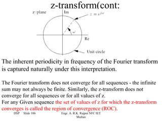
z-transform(cont:
The Fourier transform of x[n] exists if the sum ∑− x[ n ]
∞
n= ∞
converges. However, the z-transform of x[n] is just the Fourier
transform of the sequence x[n]r -n. The z-transform therefore exists
(or converge) if
X ( z ) = ∑ =−∞ x[ n]r <∞
∞ −n
n

This leads to the condition −
∑
n
<∞
∞
n= ∞
−
x[ n] z
for the existence of the z-transform. The ROC therefore consists of a
ring in the z-plane:

In specific cases the inner radius of this ring may include the origin, and the outer
radius may extend to infinity. If the ROC includes the unit circle=
DSP Slide 107 Engr. A. R.K. Rajput NFC IET z 1 , then
the Fourier transform will converge. Multan

z-transform(cont:
Most useful z-transforms can be expressed in the form
P( z )
X ( z) = ,
Q( z )
where P(z) and Q(z) are polynomials in z. The values of z for
which P(z) = 0 are called the zeros of X(z), and the values with
Q(z) = 0 are called the poles. The zeros and poles completely
specify X(z) to within a multiplicative constant.

In specific cases the inner
radius of this ring may include
the origin, and the outer radius
may extend to infinity. If the
z =
ROC includes the unit circle 1
, then the Fourier
transform will converge.

Multan

Example: right-sided exponential sequence
Consider the signal x[n] = anu[n]. This has the z-transform
∞ ∞

X ( z) = ∑a u[n]z = ∑(az )
n =−∞
n −n

n =0
−1 n

Convergence requires that ∞

∑ az −1 < ∞
n =∞

which is only the case if az − < . equivalently
1
1 or z >a .
In the ROC, the series converges to
∞
1 z
X ( z ) = ∑ (az ) = =
−1 n
, z > a,
n= 0 1 − az −1
z−a
since it is just a geometric series.
Multan

Example: right-sided exponential sequence
The z-transform has a region of convergence for any finite
value of a.

The Fourier transform of x[n] only exists if the ROC
includes the unit circle, which requires that a <1. On
the other hand, if a >1 then the ROC does not include
the unit circle, and Fourier transform does not exist. This
is consistent with the fact that for these values of a the
sequence anu[n] is exponentially growing, and the sum
therefore 110
DSP Slide does not converge.Rajput NFC IET
Engr. A. R.K.
Multan

Example: left-sided exponential sequence
Now consider the sequence x ( n) =− n u[ − − ].
a n 1
This sequence is left-sided because it is nonzero only for n ≤ 1.
−
The z-transform is ∞ −1
X ( z ) = ∑ a n u[ − − ] z −n =−∑ n z −n
− n 1 a
n= ∞
− n= ∞
−
∞ ∞
=− a −n z n = −∑a − z ) n
∑ 1 ( 1
n=1 n=0

For a − z < ,or
1
1 z <a , the series converges to

Note that the expression for the
z-transform (and the pole zero
plot) is exactly the same as for
the right-handed exponential
sequence - only the region of
convergence is different.
Specifying the ROC is therefore
critical when dealing with the z- Engr. A. R.K. Rajput NFC IET
DSP Slide 111
transform. Multan

Example: Sum of two exponentials
n n
1   1
The signal x[n] =   u[n] +  −  u[n] is the sum of two real exponentials
2  3
The z transform is
∞  −
n n
 
1  1
X ( z ) =∑  u[ n ] + −  u[ n] n
  z
n= ∞ 
−
2  3 
∞ ∞ n n
 
1  1
=∑  u[ n ] z

−n
+ ∑−  u[ n] z −

n

n= ∞ 2 
−  − 
n= ∞ 3
n n
1 −
∞ ∞
 1 −
∑
=  z  + 
n= 
1
∑− z 1 
0 2  n= 
0 3 
From the example for the right-handed exponential sequence, the first term in this
sum converges for z >1 / 2 and the second for z >1 / 3 The combined
transform X(z) therefore converges in the intersection of these regions, namely when
z >1 / 2 .  1 
2 z z − 
1 1  12 
In this case X ( z ) = + =
1 −1 1 −1  1  1
DSP Slide 112 1 − Engr. A. R.K. Rajput NFC IET
z 1+ z  z −  z + 
2 Multan 3  2  3

Example: Sum of two exponentials
The pole-zero plot and region of convergence of the signal is

Multan

Example: finite length sequence
The pole-zero plot and region of convergence of the signal is

The signal

has z transform − N−
1 −( az −1 ) n
N 1 1
X ( z ) =∑ n z −n
a =∑ az − ) n =
( 1

n=0 n=0 1 −az − 1

1 z N −a N
= .
zN−1
z −a
Since there are only a finite number of nonzero terms the sum always converges when
az −1
(a < )
,∞
is finite. There are no restrictions on and the ROC is the entire z-

plane with the exception of the origin z = 0 (where the terms in the sum are infinite). The N roots of
j ( 2πk / N )
Z k = ae
the numerator polynomial are at , k = 0,1,......N − 1
*since these values satisfy the equation ZN= aN The zero at k = 0 cancels the pole at z = a, so there are no poles except
at the origin, and the zeros are at zk = aej(2k/N) k = 1; : : : ;N -1 The zero at k = 0 cancels the pole at z = a, so there
are no poles except at 114 origin, and the zeros areA. R.K. Rajput NFC = 1; : : : ;N -1
DSP Slide the Engr. at zk = aej(2k/N) k IET
Multan

2-Properties of the region of convergence
The properties of the ROC depend on the nature of the signal. Assuming that the
signal has a finite amplitude and that the z-transform is a rational function:

The ROC is a ring or disk in the z-plane, centered on the origin
τ τ
(0 ≤ R < z < L ≤∞).
The Fourier transform of x[n] converges absolutely if and only if the ROC of
the z-transform includes the unit circle.
The ROC cannot contain any poles.
If x[n] is finite duration (ie. zero except on finite interval (∞< N1 ≤ n ≤ N 2 < ∞).
∞
), then the ROC is the entire Z-plan except perhaps at z=0 or
z= .
If x[n] is a right-sided sequence then the ROC extends outward from the
outermost finite pole to infinity.
 If x[n] is left-sided then the ROC extends inward from the innermost nonzero
pole to z = 0.
A two-sided sequence (neither left nor right-sided) has a ROC consisting of a
ring in the z-plane, bounded on the interior and exterior by a pole (and not
containing any poles).
 The ROC is115 connected region.A. R.K. Rajput NFC IET
DSP Slide a Engr.
Multan

3 - The inverse z-transform
Formally, the inverse z-transform can be performed by evaluating a
Cauchy integral. However, for discrete LTI systems simpler
methods are often sufficient.
A-Inspection method: If one is familiar with (or has a table
of) common z-transform pairs, the inverse can be found by
inspection. For example, one can invert the z-transform
 
 1  1
X ( z) = z
, >
1
 − z −
1 2,
1
 
 2 
Using Z-transform pair
1
a u[ n ] ←
n
 →
z
,........ for z > .
a
1− − az 1
By inspection we recognise that
n
 
1
x[n] =   u[ n ],
 
2

Also, if X(z) is a sum of terms then one may be able to do a term-by-
term DSP Slide 116 by inspection, A. R.K. Rajput NFC IETas a sum of terms.
inversion Engr. yielding x[n]
Multan

3 - The inverse z-transform
B-Partial fraction expansion:
For any rational function we can obtain a partial fraction expansion,
and identify the z-transform of each term. Assume that X(z) is
expressed as a ratio of polynomials in z-1:

∑
M −k
bk z
X ( z) = k =0
,
∑
N −k
ak z k =0
It is always possible to factorX(z) as
∏ (1 − c z )
M −1
b0
X(z) = k =1 k

∏ (1 − d z )
N
a0 −1
k =1 k
where the ck' s are the nonzero and poles of X(z).
Multan

The(Continue:) z-transform
Partial fraction expansion
inverse
If M<N and the poles are all first order, then X(z) can be expressed
N
as Ak
X(z) = ∑ −1
,
k =1 1 − d k z
in this case the coefficients A k are given by
( )
A k = 1 − d k z −1 X ( z )
z =d k

If M>N and the poles are first order, then an expression of the form
cab be used, and Br’s be obtained by long division of the numerator.

M-N N
Ak
X(z) = ∑B z
r =0
r
−r

1− dk z
+∑
k =1
−1
,

The A k ' s can be obtained using M < N
Multan

3 - The inverse z-transform Partial fraction expansion
The most general form for partial fraction expansion,
which can also deal with multiple - order poles, is
M-N N
Ak s
Cm
X(z) = ∑B z −r
+ ∑ +∑ .
r =0
r
k =1, k ≠ i 1− dk z −1
m =1 (1 − d z )
i
−1 m

Ways of finding the C m ' s can be found in most standard
DSP texts. The terms B r z −r correspond to shifted and
scaled impulse sequences, and invert to terms of the
form B rδ [n - r]. The fractional term s A k

1 − d k z −1
correspond to exponentia l sequences. For these terms the
ROC properties must be used to decide whether the sequences
are left - sided or right - sided.
Multan

Example: inverse by Partial fractions
Consider the sequence x[n] with z - transform

X(z) =
1 + 2z + z
−1

=
−2
1+ z
,
( )
−1 2

z > 1.
3 −1 1 −2
1− z + z
2 2
1 −1
1− z 1− z
2
−1
( )
Since M = N = 2 this can be expressed as

X(z) = B0 + A 1
+ A 2
,
−
1 −1 1−z
1
1− z
2
The value B0 can
found by be long division :
2
1 −2 3 −1 − 2 −1

2z
− z +1) z +2 z +1
2
−2 −1
z −3 z +2
−1
5z −1
−1
- 1 +5 z
X(z) =2 +

DSP Slide 120

1 −
2
1

 Engr. A.
−
(
1
 − z 1 − z R.K. Rajput NFC IET
1 )
Multan

Example: inverse by Partial fractions
The coecients A and A can be found using
A = (1 − d z ) X ( z ) d .
1 2
−1
k k z=
k
So
−1 −2
1 +2 z + z 1 +4 +4
A 1
=
1 −z
−1
−1
=
1 −2
=−9
z =1

−1 −2
1 +2 z + z 1 +2 + 1
and A = = =9
2
1 −1 1/ 2
1− z
2 z
−1
=1

9 8
There fore X(z) =2 - + −
1 −1 1 −z
1
1− z
2

Using the fact that the ROC z >1. , the terms can be inverted one at a time
by inspection to give
x[ n ] = 2δ[ n ] − 9(1 / 2) n u[ n].
Multan

C- Power Series Expansion
If Z transform is given as power series in form
∞
X (z ) = ∑ [ n] z
−n
x
n= ∞
−
2 2
=.................. +[ − ] z +x[ − ] z 1 +x[0] +x[1] z 1 +[ 2] z ......
2 1
then any value in the sequence can be found by identifying the
coefficient of the appropriate power of z-1.

Multan

Example;ZPower Series Expansion
Consider the transform
X (z ) =log ( + − )
1 az 1 , z >a
Using the power series expansion for log(1 + x), with /x/< 1, gives
∞
( −) n + a n z −
1 1 n
X (z ) =∑ ,
n=
1 n

Multan

Example; Power Series Expansion by long division
Consider the transform
1
X (z ) = , z >a
1− −
az 1
Since the ROC is the exterior of a circle, the sequence is right-sided. We therefore
divide to get a power series1in powers of z-1:
1 + az + a z
− 2 -2

X ( z ) = 1 − az −1
1
1 − az −1

−1
az
az − a z
−1 2 −2

a 2 z − 2 + .....
1
= 1 + az + a z + ........Therefore..............x[n] = a u[n].
−1 2 -2 n

1 − az −1

Multan

Example; Power Series Expansion for left-side Sequence
Consider the Z- transform
1
X (z ) = −
, z <a
1−az 1

Because of the ROC, the sequence is now a left-sided one. Thus we
divide to obtain a series in powers of z:

−
-a 1
z −a z -2 2..

−a +z z
z −a − z 2
1

az −1

Thus..............x[ n] =− n u[ − − ].
a n 1

Multan

4- Properties of the z-transform
if X(z) denotes the z-transform of a sequence x[n] and the ROC of X(z) is
indicated by Rx, then this relationship is indicated as
x[ n] ←→ ( z ),
 X
z
ROC Rx
Furthermore, with regard to nomenclature, we have two sequences such
that[ n ] ←
x1  X 1 ( z ),
z
→ ROC R x1
x2 [ n] ← X 2 ( z ),
z
→ ROC R x2
A—Linearity: The linearity property is as follows:
ax1[n] + bX 2 (n) ← z aX 1[ z ] + bX 2 ( z ),
→ ROC contains R x1 ∩ R x1 .

B—Time Shifting: The time shifting property is as follows:
x[n − n0 ] ← z z X ( z ),
→
− n0
ROC R x
(The ROC may change by the possible addition or deletion of z =0 or z = ∞.)
This is easily shown:
∞ ∞

Y ( z ) = ∑x[ n −n ] z
n =−∞ 0
−n
= ∑x[ m] z
n =−∞
− m +n0 )
(

∞

= z 126∑x[ m] z A. R.K. z NFC IET z ).
DSP
Slide
−n0
Engr.
n =−∞
= X(Rajput
Multan
−m −n0

Example: shifted exponential sequence
Consider the z-transform
1 1
X ( z) = , z >
1 4
z−
4
From the ROC, this is a right-sided sequence. Rewriting,
 
z −1  1  1
X ( z) = ,= z −1
  z >
1 −1 1 - 1 z −1  4
1− z  
4  4 
The term in brackets corresponds to an exponential sequence (1/4) nu[n]. The
factor z-1 shifts this sequence one sample to the right.
The inverse z-transform is therefore

x[n] = (1 / 4) u[n − 1] .
n −1

Multan

C- Multiplication by an exponential sequence
The exponential multiplication property is
z0 x[n] ← z X [ z / z0 ],
n
→ ROC zR,
0 x

where the notation z 0 Rx , indicates that the ROC is scaled by z (that is, 0

inner and outer radii of the ROC scale by z ). All pole-zero locations are
0

similarly scaled by a factor z0: if X(z) had a pole at z = then X(z/z0)
z 1

will have a pole at z=z0z1.
•If z0 is positive and real, this operation can be interpreted as a shrinking or
expanding of the z-plane | poles and zeros change along radial lines in the z-
plane.
If z0 is complex with unit magnitude (z0 = ejw0) then the scaling operation
corresponds to a rotation in the z-plane by and angle w 0, That is, the poles and
zeros rotate along circles centered on the origin. This can be interpreted as a
shift in the frequency domain, associated with modulation in the time domain
by ejw0n. If the Fourier transform exists, this becomes

e x[n] ← → X ( e ).
jω 0 n F j (ω − ω 0 )
Multan

Example: exponential multiplication
The z-transform pair
1
u[n] ← z
→ , z >1
1− z −1

can be used to determine the z-transform of x[n] = r n cos(w0n)u[n].
Since cos (w0n) = 1/2ejw0n + 1/2e –jw0n. The signal can be written as
u[ n] + (re )n u[ n].
1 1
x[ n ] = (r )
jω n −ω
j

2
e 0

2
0

From the exponential multiplication property,
1 1/ 2
(r e jω )n u[ n] ←
0
z
→ jω
, z >r.
2 1 −r e z −1 0

1 1/ 2
(r e−jω )n u[ n] ←
0
 z
→ −jω
, z >r .
2 1 −r e z −1 0

So
1/ 2 1/ 2
X(z) = + z >r.
1 −r e jω z −1
1 −r e−jω z −
0 1 0

1 −r cos ωz −1
0
, z >r .
DSP 1 −2r
Slide 129 cos ωz
0
−1
+r 2 z Rajput NFC IET
Engr. A. R.K.−2

Multan

D- Differentiation
The differentiation property states that
dX ( z )
nx[ n] ←z →−z
 , ROC = R x .
dz
This can be seen as follows: since
∞

∑
X ( z ) = x[ n ] z −,
n

n=
-∞

We have

dX ( z ) ∞

−z = − z ∑ (− n) x[n]z −n−1 = ∑ nx[n]z −n = z{nx[n]}.
dz n = −∞

Example: second order pole
The z-transform of the sequence x[n] = na n u[n]
Can be found 1
a u[ n] ←
n
 z
→ z >a,
1 −z −1

to be
d  1  az − 1

X(z) =-  − 
= , z >a.
DSP Slide 130
dz 1 −az  Multan −az )(1
Engr. A. R.K. Rajput NFC IET− 2
1 1

E- Conjugation
This property is
x * [n] ← z → X * ( z*),
 ROC = R x .
F- Time reversal.
1
Here x * [−n] ←z →X * (1 / z*),
 ROC = .
Rx

The notation 1/Rx means that the ROC is inverted, so if Rx is the set
of values such that rR < z <rL , then the ROC is the set of values of z su
that 1 / r l z < 1/rR .

Example: Time-reversed exponential sequence
The Signal x[ n ] = a −n u[ − ] is a time-reversed version of a nu[n]. The
n
z-transform is therefore

1 −a z −1 −1

X ( z) = = , z < a = Rx.
−1

1 − az 1 − a z
−1 −1

Multan

G- Convolution
This property state that
x1[n] * x2 [n] ← z X 1 ( z ) X 2 ( z ),
→ ROC contains R x1  R x2 .

1
Here x * [−n] ←z →X * (1 / z*),
 ROC = .
Rx
Example: evaluating a convolution using the z-transform
The z-transforms of the signal x1[n] =anu[n] and x2[n] = u[n] are
∞
1
∑
X 1 ( z) = a n z − = n
, z >a
n=0 1− az − 1

and
∞
1
.X 2 ( z) = ∑− = z n , z > 1
n= 0 1− az −
1

For a < , The z-transforms of the convolution y[n] = x 1[n] *x2[n] is
1
1 z2
Y ( z) = = z >1
(1 −az )(1 −az ) ( z −a )( z − )
−1 −1
1

1 Engr. A. R.K. Rajput NFC IET z 2
(z =
Y DSP ) Slide 132 = z >1
(1 −az )(1 −az ) ( z −a )( z − )
−1 − Multan
1
1

Example: evaluating a convolution using the z-transform

Using a partial fraction expansion,

1  1 a 
Y ( z) =  - 1 
, z >1
(1 − a ) 1 − z 1 − az 
−1 −

So
1
y ( n) = (u[n] − a n+1u[n]).
1 −a

H- Initial Value theorem
If x[n] is zero for n<0, then

x[0] = lim X ( z ).
z→∞
Multan

Some common z-transform pairs are:

Multan

I- Relationship with the Laplace transform:
Continuous-time systems and signals are usually described by the Laplace
transform. Letting z = esT , where s is the complex Laplace variable

s = =jω
d ,
we have
( d + ωT jω
z =e j )
= e e
dT T
.
Therefore
z =e dT and  z =ω =2π s =2π / ω,
T f/f ω s

where ws is the sampling frequency. As ω varies from∞ to∞, the s-plane is
mapped to the z-plane:

 The jωaxis in the s-plane is mapped to the unit circle in the z-plane.
 The left-hand s-plane is mapped to the inside of the unit circle.
The right-hand s-plane maps to the outside of the unit circle.

Multan

?
Multan

Lecture -4
Frequency Analysis

Voltage Vs Time Representation That
become
Magnitude Vs Frequency
,
Phase Vs Frequency Representation
And
Vice Versa
Multan

Frequency Analysis of Signals
•Fourier transform and Fourier series basically involve the
decomposition of the signal in terms of sinusoidal components.
With such a decomposition ,a signal is said to be represented in
the frequency domain.

•These decompositions are very important in the analysis of LTI
systems because response of a system to a sinusoidal input
signal is a sinusoid of the same frequency but of different
amplitude and phase.

•Many other decompositions of signals are possible, only the
class of sinusoidal signals possess this desirable property in
passing through a LTI system.
Multan

The Fourier Series for Continuous-Time Periodic Signals

• The Fourier Series of a periodic analogue signal x(t) is given by
∞
x (t ) = ∑ k e
j 2π 0 t
kF
c ...............................1
k= ∞
−

is a periodic signal with fundamental period Tp=1/Fo and k = 0,±1, ±2…,
We can construct periodic signals of various types by proper choice of
fundamental frequency and the coefficients CK.FO determines the fundamental
period of x(t) and coefficient Ck specify the shape of waveform. We determine the
expression for Ck
to +Tp to +Tp
− j 2πlFot  
∞

∫ x(t )e − j 2πlFot
dt = ∫ e  ∑c k e + j 2πkFot dt
to to  k =−∞ 

to +Tp to +Tp to +Tp

∫ dt = t
to
= Tp ∫ x (t )e − j 2πlFot dt = C l T p
to to

1 − j 2π 0 t
∫
kF
ck = x (t )e dt........2
Tp Tp Engr. A. R.K. Rajput NFC IET 139
Multan

• In general, the Fourier Coefficients ck are complex valued.
• If the periodic signal is real, ck and c-k are complex conjugates. As a result,
if
c k = c k e jθk

then
c − =c k e − θ
k
j k

Multan

Other forms of Fourier Series
Representation
As we have just mentioned
∞
x(t ) = ∑ c k e j2 πkF0t
k = −∞

The above equation can be re-written as

[ ]
∞
x(t ) = c0 + ∑ c k e j 2πkF0t + c − k e j 2π ( − k ) F0t
k =1

since c k = c k e jθk and c −k = c k e − jθk

[ ]
∞
∴ x(t ) = c 0 + ∑ c k e j ( 2πkF0t +θk ) + e − j ( 2πkF0t +θk )
k =1

∞
This is called the Cosine
= c0 + 2∑ c k cos( 2πkF0 tRajput NFC IET
Engr. A. R.K. + θk ) 141
k =1 Multan Fourier Series.

Other forms of Fourier Series
Representation
Yet another form for the Fourier Series can be obtained by
expanding the cosine Fourier series as
∞
x(t ) = c 0 + 2∑ c k [ cos 2πkF0 t cos θk − sin 2πkF0 t sin θk ]
k =1

Consequently, we may rewrite the above equation in
the form
∞
∴ x(t ) = a0 + ∑ ( a k cos 2π kF0 t − bk sin 2π kF0 t )
k =1

This is called the Trigonometric form of the FS,
where a0 = co, ak = 2|ck|cosθRajput NFC IET k = 2|ck|sinθ k.
Engr. A. R.K. k
and b 142
Multan

Power Density Spectrum of Periodic
Signals
A periodic signal has infinite energy and a
finite average power, which is given as
1 2
Px =
Tp ∫ x( t )
Tp
dt

If we take the complex conjugate of (1) and
substitute for x*(t), we obtain
1 ∞ ∞ 1 
∫Tp x(t )k∑∞ck e dt = ∑ ck  ∫ x(t )e
* − j 2 πkF0 t − j 2 πkF0 t
Px = *
dt 
Tp =− k=−∞  Tp Tp
 

∞ 2

=∑k
c
k= ∞
− Engr. A. R.K. Rajput NFC IET 143
Multan

Therefore, we have established the relation
∞ 2
1
∑c
2
Px =
Tp ∫ x(t )
Tp
dt =
k =−∞
k

Which is called Parse Val's relation for power signals.

This relation states that the total average power in the periodic
signal is simply the sum of the average powers in all the
harmonics.
If we plot the |ck| as a function of the frequencies kFo ,k=0,±1,±2,….
the diagram we obtain shows how the power of the periodic signal
is distributed among the various frequency components. This diagram
is called the Power Density Spectrum of the periodic signal x(t). A
typical PSD is shown in the next slide.

Multan

|ck|2

F
-2F 0 -F0 0 F0 2F 0
Power density spectrum of a continuous time periodic signal
Multan

Example1: Determine the Fourier Series and the Power
Density Spectrum of the rectangular pulse train signal
illustrated in the following figure.
x(t)

A

Tp -τ/2 τ/2 Tp
Aτ
Solution: c0 =
1
Tp ∫
τ/ 2

−τ / 2
Adt =
Tp
1 τ/ 2 Aτ sin π 0 τ
kF
and ck =
Tp ∫−τ/ 2
Ae −j2 πkF0 t dt =
Tp π 0τ
kF

where k = ±1, ±2, …..
Figure (a), (b) and (c) illustrate the Fourier
coefficients when Tp is fixed and the pulse width
τ is allowed to vary.R.K. Rajput NFC IET
Engr. A.
Multan
146

0.2
τ = 0.2Tp
0.15
0.1 Fig.(a)
0.05
0
-0.05
-60 -40 -20 0 20 40 60

0.1
τ = 0.1Tp
0.08
0.06
0.04 Fig. (b)
0.02
0
-0.02
-0.04
-60 -40 -20 0 20 40 60
Multan

0.05
0.04 τ = 0.05Tp
0.03
Fig. (c)
0.02
0.01
0
-0.01
-0.02
-60 -40 -20 0 20 40 60

From these three figures we observe that the
effect of decreasing τ while keeping Tp fixed is to
spread out the signal power over the frequency
range. The Spacing between the adjacent lines is
independent of the value of the width τ.
Multan

The following figures demonstrate the effect
of varying Tp when τ is fixed.

Multan

The figures on the previous slide ()
show that the spacing between adjacent spectral lines
decreases as Tp increases. In the limit as Tp → ∞, the
Fourier coefficients ck approach zero. This behavior is
consistent with the fact that as Tp → ∞ and τ remains
fixed, the resulting signal is no longer a power signal.
Indeed it becomes an energy signal and its average
power is zero.

The Power Density Spectrum for the rectangular pulse train is
  Aτ 
2

   , k =0
 T 
ck
2
=  p 
2 2
 Aτ   sin πkF0 τ 
 T   πkF τ  ,
    k = ±1,±2,...
 p   0 
Multan

Lecture -4
Frequency Analysis of Discrete-Time Signals

Multan

Frequency Analysis of Discrete-Time Signals
•We have already discussed the Fourier series representation for continuous-
time periodic (power) signals and the Fourier transform for finite energy
aperiodic signals.
•The frequency range for continuous-time periodic signals
extends from -∞ to ∞,that contain infinite number of frequency
components with frequency spacing (1/Tp).
•The frequency range for discrete-time signals is unique over the
interval (-π,π) or (0,2π).
• A discrete-time signal of fundamental period N can consist of
frequency components separated by 2π/N radians or f= 1/N
cycles.
•Consequently, the Fourier series representation of the discrete-
time periodic signal will contain N frequency components (the
basic difference b/w Fourier series representation for continuous-
time and discrete-time periodic signals).
Multan

The Fourier Series for Discrete-Time Signals
Suppose that we are given a periodic sequence with
period N. The Fourier series representation for x[n]
consists of N harmonically related exponential
functions
ej2πkn/N, k = 0, 1,2,…….,N-1
and is expressed as
N−1
x[n ] =∑ k e j 2 πkn / N
c
k=0

where the coefficients ck can be computed as:

1 ∞
c k = ∑ [n]e −j2 πkn / N
x
N n =0
Multan

Example: Determine the spectra of the following signals:
(a) x[n] = [1, 1, 0, 0], x[n] is periodic with period 4 (b) x[n] = cosπn/3
(c) x[n] = cos(√2)πn
Solution: (a) x[n] = [1, 1, 0, 0]
↑
N−1
1 1 3
ck = ∑ x[n]e = ∑ x[n]e
− j2πkn/ N − j2πkn/ N

N n=0 4 n=0
1 3 1 1 1
c0 = ∑ x[n] = [ x[0] + x[1] + x[2] + x[3]] = [ 1 + 1 + 0 + 0] =
4 n=0 4 4 2
Now
1 3 1 3 1
c1 = ∑x[n]e − j 2π n / 4
= ∑x[n]e − jπ n / 2 = x[0] + x[1]e − jπ / 2 + 0 + 0 
4 n =0 4 n =0 4 

1 1 1
= 1 + 1( cos 2 − j sin 2 )  = 1 + ( 0 − j )  = ( 1 − j )
π π
 4  4
4
Multan

[1 + 1 .e ]
3 3
1 1 1
c2 = ∑ x[ n ]e j2 π 2 n / 4
= ∑ x[ n ]e jπ n
= jπ

4 n= 0 4 n= 0 4
1
= [ 1 + cos π − j sin π ] = 0
4
1 3 − j2 π n 3 / 4 1 1 1
c 3 = ∑ x[n]e = [ 1 + cos( 3π / 2) − j sin( 3π / 2)] = [ 1 + 0 + j] = [ 1 + j]
4 n= 0 4 4 4
The magnitude spectra are:

c0 =
1
c1 =
4
2
c2 = 0 c3 =
4
2
2
and the phase spectra are:

Φ0=0 Φ1 =
−π
4 Φ 2 = undefined Φ3 =
π
4
Multan

(b) x[n] = cosπn/3
Solution: In this case, f0 = 1/6 and hence x[n] is periodic with
fundamental period N = 6.
Now
1 5 1 5 πn − j 2πkn / 6 1 5 πn
c k = ∑ x[n]e − j 2πkn / N
= ∑ cos e = ∑ cos e − jπkn / 3
6 n= 0 6 n= 0 3 6 n= 0 3

6 n= 0 2
[ +e e ] = ∑e
12 n = 0
+e [
1 5 1 jπ n / 3 − jπn / 3 − jπkn / 3 1 5 j π3n ( 1− k ) − j π3n ( 1+ k )
= ∑ e ]
1 5 πn 1 5 πn
∴ c0 = ∑ 2 cos = ∑ cos
12 n= 0 3 6 n= 0 3
1
= [ cos 0 + cos π3 + cos 23π + cos 33π + cos 43π + cos 53π ] = 0
6
Similarly, c2 = c3 = c4 = 0, NFC1IET c5 = ½.
Engr. A. R.K. Rajput c = 156
Multan

(c) Cos(√2)πn

Solution: The frequency f0 of the signal is 1/√2 Hz.
Since f0 is not a rational number, the signal is
not periodic. Consequently, this signal cannot be
expanded in a Fourier series.

Multan

Power density Spectrum of Periodic Signals
The average power of a discrete time periodic signal with period N is
N −1
1
∑ x ( n)
2
Px =
N n =0

The above relation may also be written as
1 N −1 1 N −1  N −1 * − 2 πkn / N 
Px = ∑ x[n]x [n] = ∑ x[n] ∑ ck e
*
 

N n=0 N n=0  n=0 
or
1
N−1 N−1

Px =∑  c *
k ∑ [n]e
x −j 2 π / N
kn

n=0 N n=0 
N−1 2 N−1
1
=∑ k ∑x[n]
2
c =
k=0 N n=0

This is Parse Val's Theorem for Discrete-Time Power Signals.
Multan

The Fourier Transform of Discrete-Time Aperiodic
Signals
The Fourier Transform of a finite energy discrete time signal x[n] is defined as

∞
X( w ) = ∑ x[n]e
n = −∞
− jwn

X(w) may be regarded as a decomposition of x[n] into its Frequency
components. It is not difficult to verify that X(w) is periodic with frequency
2π.Indeed,X(ω) is periodic with period 2π,that is,

∞
X (ω+2π ) = ∑ (n )e −j (ω 2π ) n
k x + k

n= ∞
−

∞
................... = ∑ (n )e −jω e −j 2π
x n kn

n= ∞
−

∞

∑( )
. = Multann e −jω
....................Engr. A. R.K. Rajput NFC IETn
n= ∞
−
x = X (ω) 159

• We observe two basic differences b/w the Fourier transform of a discrete-
time finite-energy signal and the Fourier transform of a finite-energy
analog signal .
• First, for continuous time signals, the spectrum of the signal have a
frequency range of (-∞,∞). In contrast, the frequency range for a discrete -
time signal is unique over the frequency interval of (-π,π).
• The second one is also a consequence of the discrete-time nature of the
signal. Since the signal is discrete in time , the Fourier transform of the
signal involves the summation of terms instead of an integral, as in the
case of continuous – time signals.
• Let us evaluate the sequence x(n) from X(ω).we multiply both sides of
X(ω) by ejωm and integrate over the interval (-π,π).
π π
 ∞ 
∫π X (ω)e
jωm
dω = ∫  ∑ x(n)e − jωn e jωm dω
− −π n =−∞ 
π
2π........m = n
∫
−π
e jω( m −n ) dω = 
 0.........m ≠ n
Multan

π
∞
2π ( n)........m = n
x
∑
n =−∞
x ( n) ∫ e jω( m −n ) dω = 
 0.........m ≠ n
−π

π
1
x (n) = ∫
2π −π
X (ω)e jωn dω

Energy Density Spectrum of Aperiodic Signals
Energy of a discrete time signal x[n] is defined as
∞ 2

Ex = ∑x[n]
n =−∞

Let us now express the energy Ex in terms of the spectral characteristic
X(w). First we have
∞ ∞
1 π ∗ 
E x = ∑ x[n]x [n] = ∑ x[n] ∫ X ( w )e − jwn dw 
*

n = −∞ n = −∞  2π −π 
If we interchange the order of integration and summation in the above
equation, we obtain
1 π ∗  ∞ − jwn  1 π 2
Ex =
2π ∫−π X (w )n∑ x[A. R.K. Rajputdw = 2π ∫−π X(w ) dw
Engr. n ]e
 =−∞ Multan  NFC IET

161

Therefore, the energy relation between x[n] and X(w) is

2 π 2
∞
1
E x = ∑ x[n] = ∫π X(w ) dw
n = −∞ 2π −

This is Parse Val's relation for discrete-time aperiodic signals.

Multan

Example: Determine and sketch the energy density
spectrum of the signal x[n] = anu[n],
-1<a<1
Solution:
( )
∞ ∞ ∞
1
∑ x[n]e− jwn = ∑ ane− jwn = ∑ ae− jw =
n
X( w ) =
n= − ∞ n= 0 n= 0 1 − ae − jw
The energy density spectrum (ESD) is given by
2 1
S xx ( w ) = X( w ) = X( w )X∗ ( w ) =
(1 − ae )(1 + ae )
− jw jw

1
X(w) =
1 − 2a cos w + a 2

a = 0.5 a= -0.5

w 163
π 0 Multan π

Example: Determine the Fourier Transform and the energy
density spectrum of the sequence
 ,
A 0 ≤n ≤L −1
x[n ] =
0, otherwise

Solution:
∞ L−1
1 − e − jwL − j( w / 2 )( L − 1 ) sin( wL / 2)
X( w ) = ∑ x[n]e − jwn = ∑ Ae − jwn
n= − ∞ 0
=A
1− e − jw
= Ae
sin( w / 2)

The magnitude of x[n] is

 A L, w =0
X( w ) = 
A sin( wL/ /22 ) , otherwise
 sin( w )

and the phase spectrum is

∠ X( w ) = ∠ A − ∠ (L − 2) + ∠ w
2
sin( wL / 2 )
sin( w / 2 )
The signal x[n] and its magnitude is plotted on the next slide. The
Phase spectrum is left as an exercise.
Multan

x[n]

|X(w)|

Multan

Properties of DTFT
Symmetry Properties:
Suppose that both the signal x[n] and its transform X(w) are complex
valued. Then they can be expressed as
x[n] = xR[n] + j xI[n] (1)

X(ω) = XR(ω) + j XI(ω) (2)
The DTFT of the signal x[n] is defined as
∞
X (ω =
) ∑x[ n]e −jω
n= ∞
−
n (3)

Substituting (1) and (2) in (3) we get
∞
X R (ω ) + jX I (ω ) = ∑ [ x R [n] + x I [n]]e − jωn
n = −∞
but
− jωn
e = cos ωn − j sin ωn
Multan

∞
∴ X R (ω ) + jX I (ω ) = ∑ [x
n = −∞
R
[n] + x I [n]].[ cos ω n − j sin ω n]

separating the real and imaginary parts, we have
∞
X R (ω) = ∑[ x
n =−∞
R [n] cos ωn + x I [ n] sin ωn ] (4)
∞
X I (ω ) = − ∑ [ x R (ω ) sin ωn − x I [n] cos ωn] (5)
n = −∞

In a similar manner, one can easily prove that
1
x R [ n] =
2π 2
∫[ X
π
R (ω) cos ωn − X I (ω) sin ωn]dω

1
x I [ n] =
2π ∫[ X
π
2
R (ω) sin ωn + X I (ω) cos ωn ]dω

Multan

DTFT Theorems and Properties
• Linearity
If x1[n] ↔ X1(w) and x2[n] ↔ X2(w), then
a1x1[n] + a2x2[n] ↔ a1X1(w) + a2X2(w)

Example 1: Determine the DTFT of the signal
x[n] = a|n| , -1< a <1
Solution: First, we observe that x[n] can be expressed as
x[n] = x1[n] + x2[n]
where

Multan

a n , n ≥ 0 a − n , n < 0
x1[n] =  and x 2 [n] = 
 0, n < 0  0, n ≥ 0

( )
∞ ∞ ∞

∑ x1[n]e = ∑a e = ∑ ae − jω
− jωn − jωn n
Now X 1 (ω) =
n

n =−∞ n =0 n =0

= 1 + ae − jω + ( ae − jω ) + ( ae − jω ) + .... =
2 3 1
1 − ae − jω

∑ ( ae )
∞ −1 −1

and X 2 (ω ) = ∑ x2 [n]e − jω n
= ∑a e − n − jω n
= jω − n

n = −∞ n = −∞ n = −∞

ae jω
( )
∞
= ∑ ae jω k
= ae jω +( ae jω ) 2 +... =
k =0 1 −ae jω
Now

1 ae jω 1− a2
X (ω ) = X 1 (ω ) + X 2 (ω ) = − jω
+ jω
=
1 − ae 1 − ae 1 − 2a cos ω + a 2
Multan

• Time Shifting
If x[n] ↔ X(ω) then x[n-k] = e-jωkX(ω)
∞
Proof: F [ x[n − k ]] =
∑
n= − ∞
x[n − k ]e − jω n

Let n – k = m or n = m+k
∞ ∞
∴ F [ x[n − k ]] = ∑ x[m]e − jω ( m + k )
= e − jwk ∑ x[m]e − jω m
= e − jω k X (ω )
m = −∞ m = −∞

• Time Reversal property
If x[n] ↔ X(ω) then x[-n] ↔ X(-ω)
Proof:
∞ −∞ ∞
F [ x[− n]] = ∑ x[− n]e − jω n
= ∑ x[m]e jω m
= ∑ x[m]e − j (− ω m)
= X (− ω )
n= − ∞ m= ∞ m= − ∞
Multan

Lecture -7

Multan

• Convolution Theorem
If x1[n] ↔ X1(ω) and x2[n] ↔ X2(ω)
then
x[n] = x1[n]*x2[n] ↔ X (ω) = X1(ω)X2(ω)
Proof: As we know[convolution formula]
∞
x[n] = x1[n] * x 2 [n] = ∑ x [k ]x [n − k ]
k=−∞
1 2

Therefore ∞ ∞
 ∞  − jω n
X (ω ) = ∑ x[n]e
n = −∞
− jω n
= ∑  ∑ x1 [k ]x 2 [n − k ]e
n = −∞  k = −∞ 
Interchanging the order of summation and making a substitution
n-k = m, we get ∞
 ∞

X (ω = ∑ 1 [ k ] ∑ 2 [ m] −jω( m +k )
) x x e
k= ∞
−  =−
m ∞ 
 ∞ −jω   ∞ m 
= ∑ 1 [ k ]e
x k
 ∑ x 2 [ m]e −jω  = X 1 (ω X 2 (ω
) )
 =−
k ∞  =−
m ∞ 

If we convolve two signal in time domain, then this is equivalent to
multiplying their spectra in frequency domain.
Multan

• Example 2: Determine the convolution of the sequences
x1[n] = x2[n] = [1, 1, 1]
As known X 1 (ω ) = X 2 (ω ) = 1 + 2 cos(ω )

Solution: ∞ 1
X 1 (ω ) = X 2 (ω ) = ∑ x [n]e
n = −∞
1
− jω n
= ∑ x [n]e
n = −1
1
− jω n

[ jω
= x1[− 1]e + x1[0] + x2 [1]e − jω
] = [e jω − jω
+ 1 + e ] = 1 + 2 cos ω
Then X(ω) = X1(ω)X2(ω) = (1 + 2cosω)2 =1 + 4cosω+ 4(cosω)2 .
= 1 + 4cosω+ 4(1+cos2ω/2) = 1 + 4cosω+ 2(1+cos2ω).
= 1 + 4cosω+ 2+2cos2ω).
= 3 + 4cos ω + 2cos2ω
= 3 + 2(ejω + e-jω) + (ej2ω + e-j2ω)
Hence the convolution of x1[n] and x2[n] is
x[n] = [1 2 3 2 1]
Multan

• The Wiener-Khintchin Theorem:
Let x[n] be a real signal. Then rxx[k] ↔Sxx(w)
In other words, the DTFT of autocorrelation function is
equal to its energy density function.*
Proof: The autocorrelation of x[n] is defined as
∞
rxx [ n] = ∑x[k ]x[k − n]
k =−∞
∞
 ∞ 
Now F [ rxx [n]] = ∑
n =−∞
∑
k =−∞
x[ k ] x[ k − n]e − jwn


Re-arranging the order of summations and making
Substitution m = k-n we get
∞
 ∞ 
F [rxx [n]] = ∑ x[k ] ∑ x[m] e − jw ( k − m )
Engr. A. R.K. Rajput NFC 
k = −∞  m = −∞ IET 174
Multan

 ∞  ∞ jω m 
=  ∑ x[k ]e −   ∑ x[m]e  = X (ω ) X (−ω ) =| X (ω ) | 2 = S xx ( ω )
jω k

 k = −∞   m = −∞ 
• Frequency Shifting:
Displacement in frequency multiplies the time/space function by a
unit phasor which has angle proportional to time/space and to the
amount of displacement.
If
x[ n] ↔ X (ω)
then
e jw0 n x[ n] ↔ X (ω −ω0 )
jω n
As from above property, multiplication of a sequence x(n) bye o
is equivalent to a frequency translation of the spectrum X(w)
by wo. So it be periodic, The shift ωo applies to the spectrum of
the signal in every period Engr. A. R.K. Rajput NFC IET 175
Multan

• The Modulation Theorem:
If x[n] ↔ X(w) then
x[n] cosω0[n] ↔ ½X(ω + ω0) + ½X(ω - ω0)
Proof: Multiplication of a time/space function by a
cosine wave splits the frequency spectrum of the
function.
Half of the spectrum shifts left and half shifts right.
This is simply a variant of the shift theorem
which makes use of Euler'sjx relationship
−
jx
e +e
∴cos( x) =
2
∞ ∞
 e jω0 n + e − jω0 n  − jωn Use
F [ x[n] cos ω 0 n] = ∑ x[n] cos ω ne
0
− jωn
= ∑ x[n] e frequenc
n = −∞ n = −∞  2  y shift
property

Multan

• The Modulation Theorem: If x[n] ↔ X(w) then
x[n] cosω0[n] ↔ ½X(ω + ω0) + ½X(ω - ω0)
Proof:

 e jω 0n + e − jω 0 n  − jω n
Use frequency shift property ∞ ∞
F [ x[n] cos ω 0 n] = ∑ x[n] cos ω 0 ne − jω n = ∑ x[n] e
n = −∞ n = −∞  2 

[ ]
∞
1
= ∑x[ n] e
− j (ω− 0 ) n
ω − j (ω+ 0 )
ω
+e
2 n =−∞
∞ ∞
= X (ω + ω 0 ) + (ω − ω 0 )
1 1 1 1
= ∑ x[n]e + ∑ x[n]e
− j (ω + ω 0 ) n − j (ω − ω 0 ) n

2 n = −∞ 2 n = −∞ 2 2

Multan

• Parseval’s Theorem:
If x1[n] ↔ X1(w) and x2[n] ↔ X2(w) then
∞ π
1
∑
n =−∞
x1 [n]x* [n] =
2 ∫
2π −π
X1 ( w ) X* ( w )dw
2

π π
1 1  ∞ − jω n  *
Proof: R.H .S . = ∫π X 1 ( ω ) X 2 ( ω ) dω = 2π −∫π  n∑−∞ x1 [ n]e  X 2 (ω )dω
*

2π − =
∞ π ∞
1
= ∑ x1 [n] ∫ X 2 (ω)e
* − jωn
dω = ∑ x1 [n]x 2 [n] = L.H .S
*

n =−∞ 2π −π n =−∞

In the special case where x1[n] = x2[n] = x[n], the Parseval’s
Theorem reduces to ∞ 2 π 2
1
∑ ( n)
x =
2π−∫ X (ω dω
)
n= ∞
− π

We observe that the LHS of the above equation is energy E x
of the Signal and Engr. A. R.K. Rajput NFC IET
the R.H.S is equal to the energy
density spectrum. Multan
178

Thus we can re-write the above equation as
∞ 2 π π
1 1
E x = ∑ [ n] ∫ X (ω dω= ∫S xx (ω dω
2
x = ) )
n= ∞
− 2π −π 2π −π

• Multiplication of two sequences: [Windowing
Theorem]
Windowing isX1(ω) process[n] ↔ X2(ω)a small subset of a larger
If x1[n] ↔ the and x2 of taking then
dataset, for processing and analysis. A naive approach, the
rectangular window, involves simply truncating the dataset before
and after the window, while not modifying the contents of the
window at all. However, as we will see, this is a poor method of
windowing and causes power leakage.
π
1
X 1 (λ)X ( − )dλ
ω λ
2π∫
x1 [ n] x 2 [ n] ↔ 2
π
−

Application of a window to a dataset will alter the spectral
properties of that dataset. In a rectangular window, for instance, all
the data points outside the window are truncated and therefore
assumed to be zero. The cut-off points atIET ends of the sample will
Engr. A. R.K. Rajput NFC
the
introduce high-frequency components Multan
179

Multiplication of two sequences: [Windowing Theorem](cont:)
If x1[n] ↔ X1(ω) and x2[n] ↔ X2(ω) then
π
1
x1 [ n] x 2 [ n] ↔
2π−∫X 1 (λX 2 (ω λdλ
π
) − )

Proof:

∞ ∞ 1 π

F [ x1[n]x2 [n]] = ∑ x [n]x [n]e
1 2
− jω n
= ∑  ∫π X 1 ( λ )e dλ  x 2 [n]e − jω n
jλ n

n= − ∞ n = −∞  2π − 
π π
1  ∞ − j (ω − λ ) n  1
=
2π −
∫π X 1 ( λ )dλ n∑ x2 [n]e
 = −∞
 = 2π
 −
∫π X ( λ ) X
1 2 (ω − λ )dλ

Show periodic Convolution
Technique use for FIR filter design

Multan

• Differentiation in the Frequency Domain:
If x[n] ↔ X(w) then Fnx[n] ↔ jdX(w)/dw
Differentiation of a function induces a 90° phase shift in the
spectrum and scales the magnitude of the spectrum in proportion
to frequency. Repeated differentiation leads to the general result:

Proof: dX (ω ) d  ∞ − jωn 
∞
d
dω
=

∑
dω n =−∞
x[ n]e  = ∑ x[n] e − jωn
 n =−∞ dω
dX (ω ) ∞
∴ = − j ∑ nx[n]e − jωn
dω n = −∞
Multiplying both sides by j we have
dX (ω) ∞
dX (ω )
j = ∑nx[ n]e − jωn OR j = F [nx[n]]
dω n =−∞ dω
This theorem explains why differentiation of a signal has the reputation
for being a noisy operation. Even if the signal is band-limited, noise will
introduce high frequency Engr. A. R.K. Rajput NFC IET are greatly amplified by
signals which
differentiation. Multan 181

The Frequency Response Function:
The response of any LTI system to an arbitrary input
signal x[n] is given by convolution sum Formula
∞
y[n ] =∑ ]x[n − ]
h[k k (6)
k =∞
−

In this I/O relationship, the system is characterized
in the time domain by its unit impulse response
h[k]. To develop a frequency domain
characterization of the system, let us excite the
system with the complex exponential
x[n] = Aejwn. -∞ < n < ∞ (7)
where A is the amplitude and w is an arbitrary frequency
confined to the frequency interval [-π, π]. By substituting
(7) into (6), we obtain the response NFC IET
Engr. A. R.K. Rajput 182
Multan

[ ]
∞
y[n] = ∑ h[k ] Ae jw ( n −k )
k = −∞
 ∞ − jwk  jwn
= A  ∑h[k ]e e
k =−∞ 
or
y[n] = AH( w )e jwn
(8)
where ∞
H( w ) = ∑h[k ]e −jwk
k =−∞
(9)

The exponential Aejwn is called an Eigen-function of
the system. An Eigen function of a system is an input
signal that produces an output that differs from the
input by a constant multiplicative factor. The
multiplicative factor is called an Eigen-value of the
System. Engr. A. R.K. Rajput NFC IET
Response is also in form of complex exponential with same frequency as input, but altered by the multiplicative factor H(w).
Multan 183

Example: Determine the magnitude and phase of H(w)
for the three point moving average(MA) system
y[n] = 1/3[x[n+1] + x[n] + x[n-1]]
Solution: since h[n] = [1/3, 1/3, 1/3]

It follows that
H(w) = 1/3(ejw +1 + e-jw) = 1/3(1 + 2cosw)
Hence
|H(w)| = 1/3|1+2cosw| and

 0, 0 ≤ w ≤ 2 π / 3
Φ (w ) = 
 π , 2π / 3 ≤ w < π
Multan

11

|H(w)|

w
0 2π/3

π
Φ(w)

w
0 2π/3
Multan

Example:An LTI system is described by
the following difference equation:
y[n] = ay[n-1] + bx[n], 0<a<1
(a) Determine the magnitude and phase of
the frequency response H(w) of the system.
(b) Choose the parameter b so that the
maximum value of |H(w)| is unity.
(c) Determine the output of the system to
the input signal
x[n] = 5 + 12sin(π/2)n – 20cos (πn + π/4)

Multan

Solution:
(a) The frequency response is
Y( w ) = ae − jw Y( w ) + bX( w )
− jw
(1 − ae )Y( w ) = bX( w )
Y( w ) b b b
H( w ) = = = =
X( w ) 1 − ae − jw
1 − a(cos w − j sin w ) ( 1 − a cos w ) − ja sin w
Now H( w ) =
b
=
b
( 1 − a cos w ) 2 + ( a sin w ) 2 1 + a 2 − 2a cos w
 a sin w 
and Φ( w ) = −tan −1  
 1 − a cos w 

These responses are sketched on the next slide.

Multan

(b) It is easy to find that |H(w)| attains its
maximum value at w = 0. At this frequency,
we have
b
H( 0) = =1 Which implies that b = ±(1-
1 −a
a).
At b = (1-a), we have
1−a a sin w
H( w ) = −1
1 + a 2 − 2a cos w and Φ( w ) = − tan 1 − a cos w

(c) The input signal consists of components of frequencies
w = 0, π/2 and π radians.
For w = 0, |H(0)| = 1 and θ(0) = 0.
For w = π/2,  π  1 − a 1 − 0.9
H  = = = 0.074.
 2 1+ a 2
1 + ( 0. 9 ) 2

 π
Θ  = − tan −1 a = − tan −1 (0.9) = −42 0
  Multan
188
2

For w = π, 1−a
| H( w ) |= = 0.053
1+ a
Θ(π ) = 0

Therefore, the output of the system is

 π  π  π   π 
y[n] = 5 H(0) + 12 H  sin  n + Θ    − 20 H( π ) cos  π n + + Θ ( π ) 
 2 2  2   4 
= 5 + 0.888 sin( n − 42 ) − 1.06 cos( π n + )
π
2
0 π
4

Multan

Response to A-periodic input signals
Consider the LTI system of the following figure
where x[n] is the input, and y[n] is the output.
x[n] y[n]
LTI System
h[n], H(w)

If h[n] is the impulse response of the system, then
y[n] = h[n]*x[n]
The corresponding frequency domain representation is
Y(w) = H(w)X(w) [
Corresponding Fourier transform of the y(n),x(n), & h(n) respectively]

Now the squared magnitude of both sides is given by
|Y(w)|2 = |H(w)|2|X(w)|2
Or
Syy(w) = |H(w)|2Sxx(w)
where Sxx(w) and Syy(w) are the energy density spectra of the
input and output signals, respectively. IET
Engr. A. R.K. Rajput NFC 190
Multan

The energy of the output signal is
π π
1 1
Ey = ∫πS yy ( w )dw = ∫π| H( w ) | S xx ( w )dw
2

2π − 2π −

Example: An LTI system is characterized by its
impulse response h[n] = (1/2)nu[n]. Determine the
spectrum and the energy density spectrum of
the output signal when the system is excited by the
signal x[n] = (1/4)nu[n].
Solution: ∞ n
1
H( w ) = ∑ ( 1 ) e − jwn =
n=0
2
1 − 1 e − jw
2

1
Similarly, X( w ) =
1 − 1 e −jw
4

Hence the spectrum of the signal at the output of the system
is Engr. A. R.K. Rajput NFC IET 191
Multan

1
Y( w ) = H( w )X( w ) =
( )(
1 − 1 e − jw 1 − 1 e − jw
2 4 )
The corresponding energy density spectrum is
2 2 2
S yy ( w ) = Y( w ) = H( w ) X( w )
1
=
( 5 − cos w )( 17 − 1 cos w )
4 16 2

Multan

DTFT and DFT
• The DTFT of an aperiodic discrete time
signal is defined as
∞ (1)
X [ w] = ∑x[ n]e − jwn

n =−∞

• The DFT of a signal is defined as
N −1
X(k ) = ∑ x[n]e − jk 2 πn / N (2)
n =0

• Inverse DFT is defined as
N −1
1
x[n] =
N
∑ X [k ]e
k =0
j 2πkn / N
(3)

What is difference between DTFT and DFT?

Multan

• The DFT is periodic with period N.
N −1
Proof: X[k ] = ∑ x[n]e − jk 2 πn / N

n=0
N− 1
X[k + N] = ∑ x[n]e − j( k + N ) 2 π n / N
n= 0
N −1
= ∑x[n]e −jk 2 πn / N e −j2 πn
n =0

Since e-j2πn = 1
N−1
∴ X[k + N] = ∑ x[n]e − jk 2 πn / N
n= 0

= X[k ]
proved
Multan

Example 1: Find the DFT of the following sequence
[1 0 0 1]
N −1 3 3
X[k ] = ∑ x[n]e − jk 2 πn / N = ∑ x[n]e − jk 2 πn / 4 = ∑ x[n]e − jkπn / 2
n=0 n=0 n=0
3
X[0] = ∑x[n] = x[0] + x[1] + x[2] + x[ 3] = 1 + 0 + 0 +1 = 2
i =0
3
X[1] = ∑x[n]e − jkπn / 2 = x[0] + 0 + 0 + x[3]e − j3 π / 2
n =0
− j3 π / 2
= 1 + 1.e = 1 + cos( 32π ) − j sin( 32π ) = 1 + j
3
X [2] = ∑ x[n]e − jπn = x[0] + x[3]e − j 3π = 1 +1.[cos(3π ) − j sin ( 3π ) ] = 0
n =0

n=0
X [3] = ∑ x[n]e − j 3πn / 2 = x[0] + x[3]e − j 9π / 2 = 1 − j
3
Multan

Example 2: Find the IDFT of the sequence
[2 1+j 0 1-j]
1 N −1
Solution: x[n] = ∑ X[k ]e jk 2πn / N
N k =0
1 N −1 1
x[0] = ∑ X[k ] = [ X[0] + X[1] + X[2] + X[3]]
Now 4 k =0 4
1 3 1 3
x[1] = ∑ X[k ]e jk 2 π / 4
= ∑ X[k ]e jkπ / 2
4 k=0 4 k =0
jπ / 2 jπ j3 π / 2
= X[0] + X[1]e + X[2]e + X[3]e =0
Similarly,

X[2] = 0 and X[3] = 1
Multan

Computational Complexity of the DFT
A large number of multiplications and
additions are required for the calculation
of the DFT.
Consider an 8-point DFT as given by
7
X[k ] = ∑ x[n]e − jk 2 πn / 8
n= 0

Let k2π/8 = K
7
x[n ] =∑ [n ]e −jKn
x
n=0

x[0]e − jK 0 + x[1]e − jK 1 + x[2]e − jK 2 + x[3]e − jK 3 + x[4]e − jK 4 +
x[5]e − jK 5 + x[6]e − jK 6 + xA.7]eRajput NFC IET
Engr. [ R.K.
− jK 7
Multan
197

There are eight complex multiplications and
seven complex additions. There are also
eight harmonic components to be evaluated.
Therefore, for an 8-point DFT:
Number of complex multiplications = 8×8
Number of complex additions = 8×7
For an N-point DFT
complex multiplications = N2
complex additions = N(N-1)
Clearly some means of reducing these is
required.
Multan

Decimation-in-time fast fourier transform
algorithm (Cooley-Tuckey Algorithm):
Notations: Equation (2) can be re-written as
n −1
X1 [k ] = ∑ x n e − j2 πnk / N (4)
N =0

Let WN = e − j2 π / N (5)

( − j 2π / N ) 2 − j 2π /( N / 2 )
Also note that W = [e
2
N ] =e = WN / 2 (6)

and WNk + N / 2 ) = WN WN / 2 = WN e − j( 2 π / N )( N / 2 )
( k N k

=W e k − jπ
N = W ( cos π − j sin π ) = − W
k
N
k
N (7)
Multan

Summary:
− j2 π / N
WN = e
W = WN / 2
2
N
(k + N / 2)
W N = −W k
N

N−1
DFT: X1 [k ] = ∑ n WN
x kn (8)
n =0

Multan

Consider n data samples as:
x0x1x2x3………xn
Divide these samples into an even
numbered and odd numbered sequenes x2n
and x2n+1 respectively.
That is,
x2n = x0x2x4…..,xN-2
x2n+1 = x1x3x5….xN-1
Both of the above sequences contain N/2
points. Engr. A. R.K. Rajput NFC IET 201
Multan

Now equation (8) can be re-written as
follows:
N / 2 −1 N / 2 −1
X1 [k ] = ∑ x 2n WNnk +
n =0
2
∑ x 2n +1 WN2n +1)k
n =0
(

N / 2−1 N / 2−1
= ∑ x 2n WN nk + WN
n=0
2 k
∑ x 2n +1 WNnk
n=0
2

since Wn2nk = WN / 2
nk

N / 2−1 N / 2−1
Therefore, X1[k ] = ∑ x 2n W
n=0
nk
N/2 +W k
N ∑
n=0
nk
x 2n + 1 WN / 2

The above equation can be re-written as

X1[k ] = X11[k ] + WN X12 [k ]
k
(9)
Multan

Considering line 6 of the table it is seen that
X 21[k ] = x 0 + w k
N/4 4x k = 0,1

Thus
X 21[0] = x 0 + x 4
while
− j2 π / 2
X 21[1] = x 0 + WN / 4 x 4 = x 0 + e x4 = x0 − x4
similarly
X 22 [0] =x 2 +x 6 X 22 [1] = x 2 − x 6
X 23 [0] =x1 +x 5 X 23 [1] = x1 − x 5
X 24 [0] =x 3 +x 7 X 24 [1] = x 3 − x 7

We observe that the values with k = 1 differ only by a sign from
those with k = 0.
Multan

Now X11[k ] = X 21[k ] + WN / 2 X 22 [k ]
k
(10)

(11)
So, X11[0] = X 21[0] + WN / 2 X 22 [0] = X 21[0] + X 22 [0]
0

− jπ / 2
X11[1] = X 21[1] + W X 22 [1] = X 21[1] + e
1
N/2 = X 21[1] − jX 22 [1] (12)

− j( 2 π / 8 ) 2× 2
X11[2] = X 21[2] + W X [2] = X 21[2] + e
2
N / 2 22 X 22 [2] = X 21[2] − X 22 [2] (13)

Now X 21[2] = x 0 + WN / 2 x 4 = x 0 + W22 x 4 = x 0 + x 4 = X 21[0]
2

and X 22 [ 2] = x 2 + WN / 4 x 6 = x 2 + x 6 = X 22 [0]
2

Hence equation (13) is equivalent to
X11 [2] = X 21[0] + X 22 [0] (14)
X11[3] = X 21[3] + WN / 2 XA. R.K. Rajput NFC IET
3
[3] (15)
Engr. 22 204
Multan

Now
X 21[3] = x 0 + WN / 4 x 4 = x 0 + e − j( 2 π / 2 ) 3 x 4 = x 0 + e − j3 π x 4 = x 0 − x 4 = X 21[1]
3

and X 22 [3] = x 2 − x 6 = X 22 [1]
Hence equation (15) is equivalent to
X11[3] = X 21[1] + e − j( 2 π / 4 ) 3 X 22 [1] = X 21[1] + jX 22 [1] (16)

Drawing these results together gives
X11 [0] = X 21 [0] + X 22 [0] = X 21 [0] + W8 X 22 [0]
0

X11 [ 2] = X 21 [0] − X 22 [0] = X 21 [0] − W8 X 22 [0]
0
(17)
X11 [1] = X 21 [1] − jX 22 [1] = X 21 [1] + W8 X 22 [1]
2

X11 [ 3] = X 21 [1] + jX 22 [1] = X 21 [1] − W8 X 22 [1]
2

The above equations are known as recomposition equations.
Multan

The number of complex additions and
multiplications involved is reduced in this way
because:
(i) the recomposition equations are expressed in
terms of powers of the recurring factor WN.
(ii) use is also made of relationships of the type
X21[2] = X21[0] and X21[3] = X 21[1] and
(iii) the presence of only sign differences in the
pairs of expressions is exploited.
The algorithm is known as the Cooley-Tukey
algorithm.
It can be shown that
Number of complex multiplications = (N/2)log2N
Multan

Lecture: Digital Signal Processing Batch 2009

More Related Content

What's hot

Viewers also liked

Similar to Lecture: Digital Signal Processing Batch 2009

Recently uploaded

Lecture: Digital Signal Processing Batch 2009