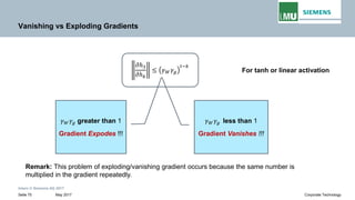
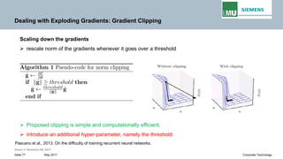
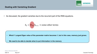
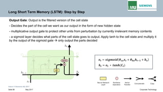
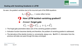
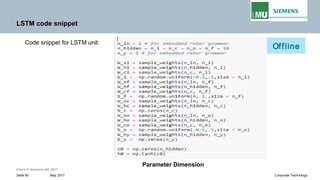
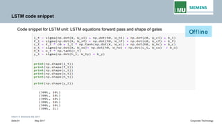
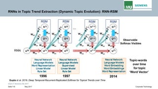
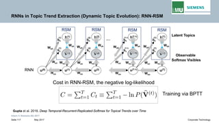
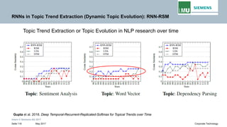
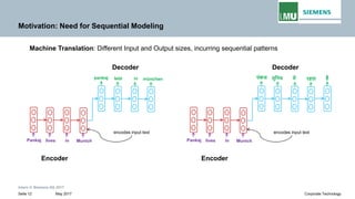
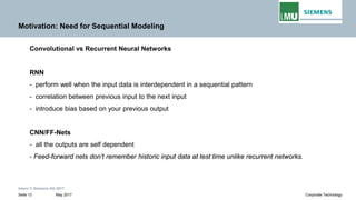
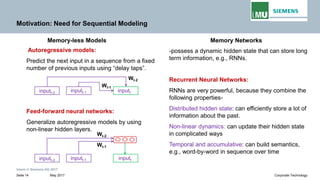
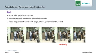
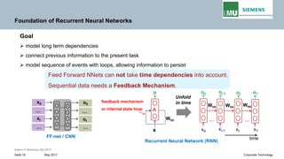
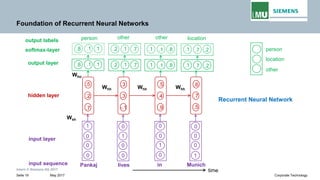
The document is a lecture by Pankaj Gupta from Siemens AG on recurrent neural networks (RNNs) covering sequence modeling, challenges in vanilla RNNs such as exploding and vanishing gradients, and various RNN variants including LSTM and GRUs. It discusses the motivation for using RNNs for tasks like speech recognition, machine translation, and sentiment classification, emphasizing the need for capturing long-term dependencies in sequential data. Additionally, it details the training process of RNNs through backpropagation through time (BPTT) and addresses the interpretability of RNNs.

1. Intern © Siemens AG 2017
Lecture-05: Recurrent Neural Networks
(Deep Learning & AI)
Speaker: Pankaj Gupta
PhD Student (Advisor: Prof. Hinrich Schütze) CIS, University of Munich (LMU)
Research Scientist (NLP/Deep Learning), Machine Intelligence, Siemens AG | Nov 2018

2. Intern © Siemens AG 2017
May 2017Seite 2 Corporate Technology
Lecture Outline
 Motivation: Sequence Modeling
 Understanding Recurrent Neural Networks (RNNs)
 Challenges in vanilla RNNs: Exploding and Vanishing gradients. Why? Remedies?
 RNN variants:
o Long Short Term Memory (LSTM) networks, Gated recurrent units (GRUs)
o Bi-directional Sequence Learning
o Recursive Neural Networks (RecNNs): TreeRNNs and TreeLSTMs
o Deep, Multi-tasking and Generative RNNs (overview)
 Attention Mechanism: Attentive RNNs
 RNNs in Practice + Applications
 Introduction to Explainability/Interpretability of RNNs

3. Intern © Siemens AG 2017
May 2017Seite 3 Corporate Technology
Motivation: Need for Sequential Modeling
Why do we need Sequential Modeling?

4. Intern © Siemens AG 2017
May 2017Seite 4 Corporate Technology
Motivation: Need for Sequential Modeling
Examples of Sequence data Input Data Output
Speech Recognition This is RNN
Machine Translation
Language Modeling
Named Entity Recognition
Sentiment Classification
Video Activity Analysis
Hello, I am Pankaj.
Hallo, ich bin Pankaj.
हैलो, म� पंकज �ं।
Recurrent neural __ based __ model network
language
Pankaj lives in Munich Pankaj lives in Munich
person location
There is nothing to like in this movie.
Punching

5. Intern © Siemens AG 2017
May 2017Seite 5 Corporate Technology
Motivation: Need for Sequential Modeling
Inputs, Outputs can be different lengths in different examples
Example:
Sentence1: Pankaj lives in Munich
Sentence2: Pankaj Gupta lives in Munich DE

6. Intern © Siemens AG 2017
May 2017Seite 6 Corporate Technology
Motivation: Need for Sequential Modeling
Inputs, Outputs can be different lengths in different examples
Example:
Sentence1: Pankaj lives in Munich
Sentence2: Pankaj Gupta lives in Munich DE
…
…
Pankaj
lives
in
Munich
PAD
PAD
person
other
other
location
other
other
Pankaj
Gupta
lives
in
Munich
Germany
person
person
other
other
location
location
…
…
FF-net / CNN
Additional word
‘PAD’ i.e., padding
FF-net / CNN
*FF-net: Feed-forward network

7. Intern © Siemens AG 2017
May 2017Seite 7 Corporate Technology
Motivation: Need for Sequential Modeling
Inputs, Outputs can be different lengths in different examples
Example:
Sentence1: Pankaj lives in Munich
Sentence2: Pankaj Gupta lives in Munich DE
…
…
Pankaj
lives
in
Munich
PAD
PAD
person
other
other
location
other
other
Pankaj
Gupta
lives
in
Munich
Germany
person
person
other
other
location
location
Pankaj lives in Munich
Pankaj Gupta lives in Munich Germany
person person other other location location
person other other location
…
…
Sequential model: RNN
Models
variable
length
sequences
FF-net / CNNFF-net / CNN
*FF-net: Feed-forward network

8. Intern © Siemens AG 2017
May 2017Seite 8 Corporate Technology
Motivation: Need for Sequential Modeling
Share Features learned across different positions or time steps
Example:
Sentence1: Market falls into bear territory  Trading/Marketing
Sentence2: Bear falls into market territory  UNK
Same uni-gram
statistics

9. Intern © Siemens AG 2017
May 2017Seite 9 Corporate Technology
Motivation: Need for Sequential Modeling
Share Features learned across different positions or time steps
Example:
Sentence1: Market falls into bear territory  Trading/Marketing
Sentence2: Bear falls into market territory  UNK
…
…
falls
bear
market
into
territory
Trading
…
…
falls
bear
market
into
territory
UNK
sentence2sentence1
No sequential
or temporal
modeling, i.e.,
order-less
Treats the two
sentences the
same
FF-net / CNN FF-net / CNN

10. Intern © Siemens AG 2017
May 2017Seite 10 Corporate Technology
Motivation: Need for Sequential Modeling
Share Features learned across different positions or time steps
Example:
Sentence1: Market falls into bear territory  Trading/Marketing
Sentence2: Bear falls into market territory  UNK
…
…
falls
bear
market
into
territory
Trading
bear falls into market territory
UNK
Sequential model: RNN
…
…
falls
bear
market
into
territory
UNK
sentence2sentence1
market falls into bear territory
Trading
Language
concepts,
Word
ordering,
Syntactic &
semantic
information
FF-net / CNN FF-net / CNN

11. Intern © Siemens AG 2017
May 2017Seite 11 Corporate Technology
Motivation: Need for Sequential Modeling
Share Features learned across different positions or time steps
Example:
Sentence1: Market falls into bear territory  Trading/Marketing
Sentence2: Bear falls into market territory  UNK
…
…
falls
bear
market
into
territory
Trading
bear falls into market territory
UNK
Sequential model: RNN
…
…
falls
bear
market
into
territory
UNK
sentence2sentence1
market falls into bear territory
Trading
Language
concepts,
Word
ordering,
Syntactic &
semantic
information
FF-net / CNN FF-net / CNN
Direction of
information flow
matters!

12. Intern © Siemens AG 2017
May 2017Seite 12 Corporate Technology
Motivation: Need for Sequential Modeling
Machine Translation: Different Input and Output sizes, incurring sequential patterns
Pankaj lives in Munich
pankaj lebt in münchen
Encoder
Decoder
encodes input text
Pankaj lives in Munich
पंकज मुिनच म� रहता
Encoder
Decoder
encodes input text
है

13. Intern © Siemens AG 2017
May 2017Seite 13 Corporate Technology
Motivation: Need for Sequential Modeling
Convolutional vs Recurrent Neural Networks
RNN
- perform well when the input data is interdependent in a sequential pattern
- correlation between previous input to the next input
- introduce bias based on your previous output
CNN/FF-Nets
- all the outputs are self dependent
- Feed-forward nets don’t remember historic input data at test time unlike recurrent networks.

14. Intern © Siemens AG 2017
May 2017Seite 14 Corporate Technology
Motivation: Need for Sequential Modeling
Memory-less Models Memory Networks
Autoregressive models:
Predict the next input in a sequence from a fixed
number of previous inputs using “delay taps”.
Feed-forward neural networks:
Generalize autoregressive models by using
non-linear hidden layers.
inputt-2 inputt-1 inputt
Wt-2
Wt-1
inputt-2 inputt-1 inputt
Wt-2
Wt-1
-possess a dynamic hidden state that can store long
term information, e.g., RNNs.
Recurrent Neural Networks:
RNNs are very powerful, because they combine the
following properties-
Distributed hidden state: can efficiently store a lot of
information about the past.
Non-linear dynamics: can update their hidden state
in complicated ways
Temporal and accumulative: can build semantics,
e.g., word-by-word in sequence over time

15. Intern © Siemens AG 2017
May 2017Seite 15 Corporate Technology
Notations
• 𝒉𝒉𝑡𝑡: Hidden Unit
• 𝒙𝒙𝑡𝑡: Input
• 𝒐𝒐𝑡𝑡 : Output
• 𝑾𝑾ℎℎ : Shared Weight Parameter
• 𝑾𝑾ℎ𝑜𝑜 : Parameter weight between hidden layer and output
• 𝜃𝜃: parameter in general
• 𝑔𝑔𝜃𝜃 : non linear function
• 𝐿𝐿𝑡𝑡 :Loss between the RNN outputs and the true output
• 𝐸𝐸𝑡𝑡 : cross entropy loss

16. Intern © Siemens AG 2017
May 2017Seite 16 Corporate Technology
Long Term and Short Dependencies
Short Term Dependencies
 need recent information to perform the present task.
For example in a language model, predict the next word based on the previous ones.
“the clouds are in the ?”  ‘sky’
 Easier to predict ‘sky’ given the context, i.e., short term dependency
 Consider longer word sequence “I grew up in France…........…………………… I speak fluent French.”
 Recent information suggests that the next word is probably the name of a language, but if we want to
narrow down which language, we need the context of France, from further back.
Long Term Dependencies
“the clouds are in the sky”

17. Intern © Siemens AG 2017
May 2017Seite 17 Corporate Technology
Foundation of Recurrent Neural Networks
Goal
 model long term dependencies
 connect previous information to the present task
 model sequence of events with loops, allowing information to persist
punching

18. Intern © Siemens AG 2017
May 2017Seite 18 Corporate Technology
Foundation of Recurrent Neural Networks
Goal
 model long term dependencies
 connect previous information to the present task
 model sequence of events with loops, allowing information to persist
Feed Forward NNets can not take time dependencies into account.
Sequential data needs a Feedback Mechanism.
feedback mechanism
or internal state loop
o
x
A
x0
…
…
FF-net / CNN
xt
…
…
o0
ot
…
…
x0
Recurrent Neural Network (RNN)
xt-1 xt xT
… …
o0 ot-1 ot oT
Unfold
in time
time
Whh Whh Whh
Whh

19. Intern © Siemens AG 2017
May 2017Seite 19 Corporate Technology
Foundation of Recurrent Neural Networks
Recurrent Neural Network
Whh
time
1
0
0
0
0
1
0
0
0
0
1
0
0
0
0
1
.8 .1 .2.1 .1 .7 .1 .1 .8 .1 .7 .2
person other other location
person
other
location
Pankaj lives in Munich
output labels
.8 .1 .2.1 .1 .7 .1 .1 .8 .1 .7 .2
softmax-layer
output layer
hidden layer
input layer
input sequence
Whh Whh
Wxh
Who
.5
.3.2
.7
.3
-.1
.5
.4
.9 .5
.6
.7

20. Intern © Siemens AG 2017
May 2017Seite 20 Corporate Technology
(Vanilla) Recurrent Neural Network
Process a sequence of vectors x by applying a recurrence at every time step:
o
x
A
x0
Vanilla Recurrent Neural Network (RNN)
xt-1 xt xT
… …
o0 ot-1 ot oT
Whh
Whh
Whh Whh
Unfold
in time
time
feedback mechanism
or internal state loop
new hidden
state at time
step, t
some function with
parameters
Input vector at time step, t
old hidden state
at time step, t-1
Remark: The same function g and same set of parameters W are used at every time step
Wxh
Who
ℎ𝑡𝑡 = 𝑔𝑔𝜃𝜃(ℎ𝑡𝑡−1, 𝑥𝑥𝑡𝑡)
h0 ht
Whh Wxh

21. Intern © Siemens AG 2017
May 2017Seite 21 Corporate Technology
(Vanilla) Recurrent Neural Network
Process a sequence of vectors x by applying a recurrence at every time step:
o
x
A
x0
Vanilla Recurrent Neural Network (RNN)
xt-1 xt xT
… …
o0 ot-1 ot oT
Whh
Whh
Whh Whh
Unfold
in time
time
feedback mechanism
or internal state loop
Wxh
Who
Remark: RNN‘s can be seen as selective summarization of input sequence in a fixed-size
state/hidden vector via a recursive update.
ℎ𝑡𝑡 = 𝑔𝑔𝜃𝜃 ℎ𝑡𝑡−1, 𝑥𝑥𝑡𝑡
ℎ𝑡𝑡 = tanh(𝑊𝑊ℎℎ ℎ𝑡𝑡−1 + 𝑊𝑊𝑥𝑥ℎ 𝑥𝑥𝑡𝑡)
𝑜𝑜𝑡𝑡 = 𝑠𝑠𝑠𝑠𝑠𝑠𝑠𝑠𝑠𝑠𝑠𝑠𝑠𝑠(𝑊𝑊ℎ𝑜𝑜ℎ𝑡𝑡)

22. Intern © Siemens AG 2017
May 2017Seite 22 Corporate Technology
Recurrent Neural Network: Probabilistic Interpretation
RNN as a generative model
 induces a set of procedures to model
the conditional distribution of xt+1 given x<=t
for all t = 1, …,T
 Think of the output as the probability distribution of the
xt given the previous ones in the sequence
Training: Computing probability of the sequence and Maximum likelihood training
x0
Generative Recurrent Neural Network (RNN)
xt-1 xt xT
… …
x1 xt xt+1
<eos>
time
<bos>
…
x0
Details: https://www.cs.cmu.edu/~epxing/Class/10708-17/project-reports/project10.pdf
Whh Whh Whh Whh

23. Intern © Siemens AG 2017
May 2017Seite 23 Corporate Technology
RNN: Computational Graphs
Initial
State, A0
𝑥𝑥1 𝑥𝑥2 𝑥𝑥3
Sequence of Inputs
𝜃𝜃
𝑔𝑔𝜃𝜃
Next state
𝑜𝑜1 𝑜𝑜2 𝑜𝑜3
Sequence of output
𝑔𝑔𝜃𝜃 𝑔𝑔𝜃𝜃

24. Intern © Siemens AG 2017
May 2017Seite 24 Corporate Technology
RNN: Different Computational Graphs
One to one
Many to One
Many to Many
𝒙𝒙𝟏𝟏
𝒐𝒐𝟏𝟏
One to Many
𝒙𝒙𝟏𝟏
Many to Many
𝒐𝒐𝟏𝟏 𝒐𝒐𝟐𝟐 𝒐𝒐𝟑𝟑
𝒙𝒙𝟏𝟏 𝒙𝒙𝟐𝟐 𝒙𝒙𝟑𝟑 𝒙𝒙𝟒𝟒
𝒐𝒐𝟏𝟏
𝒙𝒙𝟏𝟏 𝒙𝒙𝟐𝟐 𝒙𝒙𝟑𝟑 𝒙𝒙𝟒𝟒
𝒙𝒙𝟏𝟏 𝒙𝒙𝟐𝟐
𝒐𝒐𝟏𝟏 𝒐𝒐𝟐𝟐
𝒐𝒐𝟐𝟐𝒐𝒐𝟏𝟏 𝒐𝒐𝟑𝟑 𝒐𝒐𝟒𝟒

25. Intern © Siemens AG 2017
May 2017Seite 25 Corporate Technology
Backpropogation through time (BPTT) in RNN
 Training recurrent networks via BPTT
 Compute gradients via backpropagation on the (multi-layer) unrolled model

26. Intern © Siemens AG 2017
May 2017Seite 26 Corporate Technology
Backpropogation through time (BPTT) in RNN
 Training recurrent networks via BPTT
 Compute gradients via backpropagation on the (multi-layer) unrolled model
 Think of the recurrent net as a layered,
feed-forward net with shared weights and
then train the feed-forward net in time domain
Lecture from the course Neural Networks for Machine Learning

27. Intern © Siemens AG 2017
May 2017Seite 27 Corporate Technology
Backpropogation through time (BPTT) in RNN
 Training recurrent networks via BPTT
 Compute gradients via backpropagation on the (multi-layer) unrolled model
 Think of the recurrent net as a layered,
feed-forward net with shared weights and
then train the feed-forward net in time domain
Training algorithm in time domain:
 The forward pass builds up a stack of the activities of all the
units at each time step
 The backward pass peels activities off the stack to compute the
error derivatives at each time step.
 After the backward pass we add together the derivatives at all
the different times for each weight.
Lecture from the course Neural Networks for Machine Learning

28. Intern © Siemens AG 2017
May 2017Seite 28 Corporate Technology
Backpropogation through time (BPTT) in RNN
 Training recurrent networks via BPTT
 Compute gradients via backpropagation on the (multi-layer) unrolled model
 Think of the recurrent net as a layered,
feed-forward net with shared weights and
then train the feed-forward net in time domain
Training algorithm in time domain:
 The forward pass builds up a stack of the activities of all the
units at each time step
 The backward pass peels activities off the stack to compute the
error derivatives at each time step.
 After the backward pass we add together the derivatives at all
the different times for each weight.
Forward through entire sequence  compute loss
Backward through entire sequence  compute gradient
Lecture from the course Neural Networks for Machine Learning

29. Intern © Siemens AG 2017
May 2017Seite 29 Corporate Technology
Backpropogation through time (BPTT) in RNN
 Training recurrent networks via BPTT
The output at time t=T is dependent on the inputs from t=T to t=1
𝒐𝒐𝟐𝟐 𝒐𝒐𝟑𝟑
𝒐𝒐𝟏𝟏
𝐸𝐸1 𝐸𝐸2 𝐸𝐸3
𝒙𝒙𝟏𝟏 𝒙𝒙𝟐𝟐 𝒙𝒙𝟑𝟑
𝒉𝒉𝟏𝟏 𝒉𝒉𝟐𝟐 𝒉𝒉𝟑𝟑
Direction of Forward pass

30. Intern © Siemens AG 2017
May 2017Seite 30 Corporate Technology
Backpropogation through time (BPTT) in RNN
 Training recurrent networks via BPTT
The output at time t=T is dependent on the inputs from t=T to t=1
𝒐𝒐𝟐𝟐 𝒐𝒐𝟑𝟑
𝒐𝒐𝟏𝟏
𝐸𝐸1 𝐸𝐸2 𝐸𝐸3
𝒙𝒙𝟏𝟏 𝒙𝒙𝟐𝟐 𝒙𝒙𝟑𝟑
𝒉𝒉𝟏𝟏 𝒉𝒉𝟐𝟐 𝒉𝒉𝟑𝟑
Direction of Forward pass

31. Intern © Siemens AG 2017
May 2017Seite 31 Corporate Technology
Backpropogation through time (BPTT) in RNN
 Training recurrent networks via BPTT
The output at time t=T is dependent on the inputs from t=T to t=1
𝒐𝒐𝟐𝟐 𝒐𝒐𝟑𝟑
𝒐𝒐𝟏𝟏
𝐸𝐸1 𝐸𝐸2 𝐸𝐸3
𝒙𝒙𝟏𝟏 𝒙𝒙𝟐𝟐 𝒙𝒙𝟑𝟑
𝒉𝒉𝟏𝟏 𝒉𝒉𝟐𝟐 𝒉𝒉𝟑𝟑
Direction of Forward pass

32. Intern © Siemens AG 2017
May 2017Seite 32 Corporate Technology
Backpropogation through time (BPTT) in RNN
 Training recurrent networks via BPTT
The output at time t=T is dependent on the inputs from t=T to t=1
𝒐𝒐𝟐𝟐 𝒐𝒐𝟑𝟑
𝒐𝒐𝟏𝟏
𝐸𝐸1 𝐸𝐸2 𝐸𝐸3
𝒙𝒙𝟏𝟏 𝒙𝒙𝟐𝟐 𝒙𝒙𝟑𝟑
𝒉𝒉𝟏𝟏 𝒉𝒉𝟐𝟐 𝒉𝒉𝟑𝟑
Direction of Forward pass

33. Intern © Siemens AG 2017
May 2017Seite 33 Corporate Technology
Backpropogation through time (BPTT) in RNN
 Training recurrent networks via BPTT
The output at time t=T is dependent on the inputs from t=T to t=1
𝒐𝒐𝟐𝟐 𝒐𝒐𝟑𝟑
𝒐𝒐𝟏𝟏
𝐸𝐸1 𝐸𝐸2 𝐸𝐸3
𝒙𝒙𝟏𝟏 𝒙𝒙𝟐𝟐 𝒙𝒙𝟑𝟑
𝒉𝒉𝟏𝟏 𝒉𝒉𝟐𝟐 𝒉𝒉𝟑𝟑
Direction of Forward pass

34. Intern © Siemens AG 2017
May 2017Seite 34 Corporate Technology
Backpropogation through time (BPTT) in RNN
 Training recurrent networks via BPTT
The output at time t=T is dependent on the inputs from t=T to t=1
Direction of Backward pass (via partial derivatives)
--- gradient flow ---
𝒐𝒐𝟐𝟐 𝒐𝒐𝟑𝟑
𝒐𝒐𝟏𝟏
𝐸𝐸1 𝐸𝐸2 𝐸𝐸3
𝒙𝒙𝟏𝟏 𝒙𝒙𝟐𝟐 𝒙𝒙𝟑𝟑
𝒉𝒉𝟏𝟏 𝒉𝒉𝟐𝟐 𝒉𝒉𝟑𝟑
𝜕𝜕𝐸𝐸3
𝜕𝜕ℎ3
𝜕𝜕𝐸𝐸2
𝜕𝜕ℎ2
𝜕𝜕𝐸𝐸1
𝜕𝜕ℎ1
𝜕𝜕ℎ2
𝜕𝜕ℎ1
𝜕𝜕ℎ3
𝜕𝜕ℎ2

35. Intern © Siemens AG 2017
May 2017Seite 35 Corporate Technology
Backpropogation through time (BPTT) in RNN
 Training recurrent networks via BPTT
 Let us take our loss/error function to be cross entropy:
The output at time t=T is dependent on the inputs from t=T to t=1
Direction of Backward pass (via partial derivatives)
--- gradient flow ---
𝐸𝐸𝑡𝑡 𝑜𝑜𝑡𝑡′, 𝑜𝑜𝑡𝑡 = −𝑜𝑜𝑡𝑡′ log 𝑜𝑜𝑡𝑡
𝐸𝐸 𝑜𝑜𝑡𝑡′, 𝑜𝑜𝑡𝑡 = �
𝑡𝑡
𝐸𝐸𝑡𝑡(𝑜𝑜𝑡𝑡′, 𝑜𝑜𝑡𝑡)
𝐸𝐸 𝑜𝑜𝑡𝑡
′
, 𝑜𝑜𝑡𝑡 = − �
𝑡𝑡
𝑜𝑜𝑡𝑡′ log 𝑜𝑜𝑡𝑡
Where 𝑜𝑜𝑡𝑡′ are the truth values
𝒐𝒐𝟐𝟐 𝒐𝒐𝟑𝟑
𝒐𝒐𝟏𝟏
𝐸𝐸1 𝐸𝐸2 𝐸𝐸3
𝒙𝒙𝟏𝟏 𝒙𝒙𝟐𝟐 𝒙𝒙𝟑𝟑
𝒉𝒉𝟏𝟏 𝒉𝒉𝟐𝟐 𝒉𝒉𝟑𝟑
𝜕𝜕𝐸𝐸3
𝜕𝜕ℎ3
𝜕𝜕𝐸𝐸2
𝜕𝜕ℎ2
𝜕𝜕𝐸𝐸1
𝜕𝜕ℎ1
𝜕𝜕ℎ2
𝜕𝜕ℎ1
𝜕𝜕ℎ3
𝜕𝜕ℎ2

36. Intern © Siemens AG 2017
May 2017Seite 36 Corporate Technology
Backpropogation through time (BPTT) in RNN
The output at time t=3 is dependent on the inputs from t=3 to t=1
𝜕𝜕𝐸𝐸
𝜕𝜕θ
= �
1≤𝑡𝑡≤3
𝜕𝜕𝐸𝐸𝑡𝑡
𝜕𝜕θ
𝜕𝜕𝐸𝐸3
𝜕𝜕𝑊𝑊ℎ𝑜𝑜
=
𝜕𝜕𝐸𝐸3
𝜕𝜕𝑜𝑜3
𝜕𝜕𝑜𝑜3
𝜕𝜕𝑊𝑊ℎ𝑜𝑜
=
𝜕𝜕𝐸𝐸3
𝜕𝜕𝑜𝑜3
𝜕𝜕𝑜𝑜3
𝜕𝜕𝑧𝑧3
𝜕𝜕𝑧𝑧3
𝜕𝜕𝑊𝑊ℎ𝑜𝑜
Direction of Backward pass (via partial derivatives)
--- gradient flow ---
𝒐𝒐𝟐𝟐 𝒐𝒐𝟑𝟑
𝒐𝒐𝟏𝟏
𝐸𝐸1 𝐸𝐸2 𝐸𝐸3
𝒙𝒙𝟏𝟏 𝒙𝒙𝟐𝟐 𝒙𝒙𝟑𝟑
𝒉𝒉𝟏𝟏 𝒉𝒉𝟐𝟐 𝒉𝒉𝟑𝟑
𝜕𝜕𝐸𝐸3
𝜕𝜕ℎ3
𝜕𝜕𝐸𝐸2
𝜕𝜕ℎ2
𝜕𝜕𝐸𝐸1
𝜕𝜕ℎ1
𝜕𝜕ℎ2
𝜕𝜕ℎ1
𝜕𝜕ℎ3
𝜕𝜕ℎ2
WhoWho
Who
Whh Whh
Writing gradients in a sum-of-products form
𝑤𝑤ℎ𝑒𝑒𝑒𝑒𝑒𝑒, 𝑧𝑧3 = 𝑊𝑊ℎ𝑜𝑜ℎ3
𝜕𝜕𝐸𝐸3
𝜕𝜕𝑊𝑊ℎ𝑜𝑜
= 𝑜𝑜3′(𝑜𝑜3 − 1) × (ℎ3)
𝑤𝑤ℎ𝑒𝑒𝑒𝑒𝑒𝑒, ×= 𝑜𝑜𝑜𝑜𝑜𝑜𝑜𝑜𝑜𝑜 𝑝𝑝𝑝𝑝𝑝𝑝𝑝𝑝𝑝𝑝𝑝𝑝𝑝𝑝
𝜕𝜕𝐸𝐸3
𝜕𝜕𝑊𝑊ℎ𝑜𝑜
𝑑𝑑𝑑𝑑𝑑𝑑𝑑𝑑𝑑𝑑𝑑𝑑𝑑𝑑 𝑜𝑜𝑜𝑜𝑜𝑜𝑜𝑜 𝑜𝑜𝑜𝑜 𝑜𝑜3 , 𝑜𝑜3
′
𝑎𝑎𝑎𝑎𝑎𝑎 ℎ3
i.e., 𝑜𝑜3 with softmax

37. Intern © Siemens AG 2017
May 2017Seite 37 Corporate Technology
Backpropogation through time (BPTT) in RNN
𝜕𝜕𝐸𝐸3
𝜕𝜕𝑊𝑊ℎ𝑜𝑜
= 𝑜𝑜3′(𝑜𝑜3 − 1) × (ℎ3) How ?
Proof
offline
𝐸𝐸3 𝑜𝑜3′, 𝑜𝑜3 = −𝑜𝑜3′ log 𝑜𝑜3
𝜕𝜕𝐸𝐸3
𝜕𝜕𝑧𝑧3
= −𝑜𝑜3′
𝜕𝜕log(𝑜𝑜3)
𝜕𝜕𝑧𝑧3
𝑜𝑜3 = 𝑠𝑠𝑠𝑠𝑠𝑠𝑠𝑠 𝑠𝑠𝑠𝑠𝑠𝑠(𝑧𝑧3), 𝑎𝑎𝑎𝑎𝑎𝑎 𝑧𝑧3 = 𝑊𝑊ℎ𝑜𝑜ℎ3
𝑜𝑜3 =
1
Ω
𝑒𝑒 𝑧𝑧3 and , Ω = ∑𝑖𝑖 𝑒𝑒 𝑧𝑧𝑖𝑖 log o3 = z3 − log Ω
𝜕𝜕log(𝑜𝑜3)
𝜕𝜕𝑧𝑧3
= 1 −
1
Ω
𝜕𝜕Ω
𝜕𝜕𝑧𝑧3
𝜕𝜕Ω
𝜕𝜕𝑧𝑧3
= �
𝑖𝑖
𝑒𝑒 𝑧𝑧𝑧𝑧
𝛿𝛿𝑖𝑖3 = 𝑒𝑒 𝑧𝑧𝑘𝑘
𝜕𝜕log(𝑜𝑜3)
𝜕𝜕𝑧𝑧3
= 1 − 𝑜𝑜3 𝜕𝜕𝑜𝑜3
𝜕𝜕𝑧𝑧3
= 𝑜𝑜3(1 − 𝑜𝑜3)
𝜕𝜕𝐸𝐸3
𝜕𝜕𝑧𝑧3
= −𝑜𝑜3′(1 − 𝑜𝑜3) = 𝑜𝑜3
′
𝑜𝑜3 − 1 𝜕𝜕𝐸𝐸3
𝜕𝜕𝑊𝑊ℎ𝑜𝑜
=
𝜕𝜕𝐸𝐸3
𝜕𝜕𝑜𝑜3
𝜕𝜕𝑜𝑜3
𝜕𝜕𝑧𝑧3
𝜕𝜕𝑧𝑧3
𝜕𝜕𝑊𝑊ℎ𝑜𝑜
=
𝜕𝜕𝐸𝐸3
𝜕𝜕𝑧𝑧3
𝜕𝜕𝑧𝑧3
𝜕𝜕𝑊𝑊ℎ𝑜𝑜
= 𝑜𝑜3
′
𝑜𝑜3 − 1 × (ℎ3)
1. http://www.wildml.com/2015/10/recurrent-neural-networks-tutorial-part-3-backpropagation-through-time-and-vanishing-gradients/
2. https://stats.stackexchange.com/questions/235528/backpropagation-with-softmax-cross-entropy

38. Intern © Siemens AG 2017
May 2017Seite 38 Corporate Technology
Backpropogation through time (BPTT) in RNN
The output at time t=3 is dependent on the inputs from t=3 to t=1
𝜕𝜕𝐸𝐸
𝜕𝜕θ
= �
1≤𝑡𝑡≤3
𝜕𝜕𝐸𝐸𝑡𝑡
𝜕𝜕θ
𝜕𝜕𝐸𝐸3
𝜕𝜕Wℎℎ
=
𝜕𝜕𝐸𝐸3
𝜕𝜕ℎ3
𝜕𝜕ℎ3
𝜕𝜕Wℎℎ
Direction of Backward pass (via partial derivatives)
--- gradient flow ---
𝒐𝒐𝟐𝟐 𝒐𝒐𝟑𝟑
𝒐𝒐𝟏𝟏
𝐸𝐸1 𝐸𝐸2 𝐸𝐸3
𝒙𝒙𝟏𝟏 𝒙𝒙𝟐𝟐 𝒙𝒙𝟑𝟑
𝒉𝒉𝟏𝟏 𝒉𝒉𝟐𝟐 𝒉𝒉𝟑𝟑
𝜕𝜕𝐸𝐸3
𝜕𝜕ℎ3
𝜕𝜕𝐸𝐸2
𝜕𝜕ℎ2
𝜕𝜕𝐸𝐸1
𝜕𝜕ℎ1
𝜕𝜕ℎ2
𝜕𝜕ℎ1
𝜕𝜕ℎ3
𝜕𝜕ℎ2
WhoWho
Who
Whh Whh
Writing gradients in a sum-of-products form
Since ℎ3 depends on ℎ2 𝐚𝐚𝐚𝐚𝐚𝐚 ℎ2 depends on ℎ1, therefore
𝜕𝜕𝐸𝐸3
𝜕𝜕Wℎℎ
= �
𝑘𝑘=1
3
𝜕𝜕𝐸𝐸3
𝜕𝜕ℎ3
𝜕𝜕ℎ3
𝜕𝜕ℎ𝑘𝑘
𝜕𝜕ℎ𝑘𝑘
𝜕𝜕Wℎℎ
𝜕𝜕𝐸𝐸𝑡𝑡
𝜕𝜕Wℎℎ
= �
1≤𝑘𝑘≤𝑡𝑡
𝜕𝜕𝐸𝐸𝑡𝑡
𝜕𝜕ℎ𝑡𝑡
𝜕𝜕ℎ𝑡𝑡
𝜕𝜕ℎ𝑘𝑘
𝜕𝜕ℎ𝑘𝑘
𝜕𝜕Wℎℎ
e.g.,
In general,
𝜕𝜕ℎ3
𝜕𝜕h1
=
𝜕𝜕ℎ3
𝜕𝜕ℎ2
𝜕𝜕ℎ2
𝜕𝜕ℎ1

39. Intern © Siemens AG 2017
May 2017Seite 39 Corporate Technology
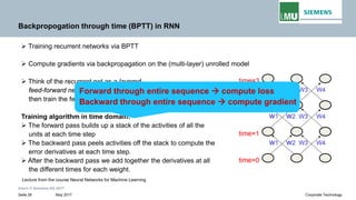
𝒐𝒐𝟐𝟐 𝒐𝒐𝟑𝟑
𝒐𝒐𝟏𝟏
𝐸𝐸1 𝐸𝐸2 𝐸𝐸3
𝒙𝒙𝟏𝟏 𝒙𝒙𝟐𝟐 𝒙𝒙𝟑𝟑
𝒉𝒉𝟏𝟏 𝒉𝒉𝟐𝟐 𝒉𝒉𝟑𝟑
𝜕𝜕𝐸𝐸3
𝜕𝜕ℎ3
𝜕𝜕𝐸𝐸2
𝜕𝜕ℎ2
𝜕𝜕𝐸𝐸1
𝜕𝜕ℎ1
𝜕𝜕ℎ3
𝜕𝜕ℎ2
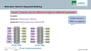
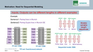
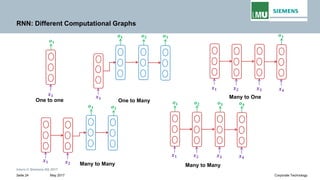
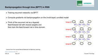
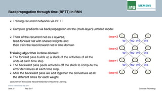
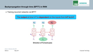
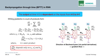
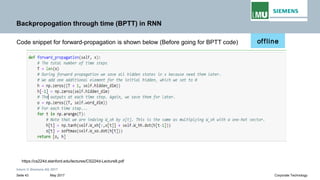
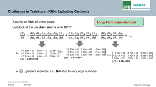
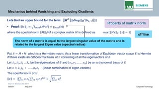
Backpropogation through time (BPTT) in RNN
The output at time t=3 is dependent on the inputs from t=3 to t=1
𝜕𝜕𝐸𝐸
𝜕𝜕θ
= �
1≤𝑡𝑡≤3
𝜕𝜕𝐸𝐸𝑡𝑡
𝜕𝜕θ
𝜕𝜕𝐸𝐸3
𝜕𝜕Wℎℎ
=
𝜕𝜕𝐸𝐸3
𝜕𝜕ℎ3
𝜕𝜕ℎ3
𝜕𝜕Wℎℎ
Direction of Backward pass (via partial derivatives)
--- gradient flow ---
WhoWho
Who
Whh Whh
Writing gradients in a sum-of-products form
Since ℎ3 depends on ℎ2 𝐚𝐚𝐚𝐚𝐚𝐚 ℎ2 depends on ℎ1, therefore
𝜕𝜕𝐸𝐸3
𝜕𝜕Wℎℎ
= �
𝑘𝑘=1
3
𝜕𝜕𝐸𝐸3
𝜕𝜕ℎ3
𝜕𝜕ℎ3
𝜕𝜕ℎ𝑘𝑘
𝜕𝜕ℎ𝑘𝑘
𝜕𝜕Wℎℎ
𝜕𝜕𝐸𝐸𝑡𝑡
𝜕𝜕Wℎℎ
= �
1≤𝑘𝑘≤𝑡𝑡
𝜕𝜕𝐸𝐸𝑡𝑡
𝜕𝜕ℎ𝑡𝑡
𝜕𝜕ℎ𝑡𝑡
𝜕𝜕ℎ𝑘𝑘
𝜕𝜕ℎ𝑘𝑘
𝜕𝜕Wℎℎ
𝜕𝜕ℎ𝑡𝑡
𝜕𝜕h𝑘𝑘
= �
𝑡𝑡≥𝑖𝑖>𝑘𝑘
𝜕𝜕ℎ𝑖𝑖
𝜕𝜕ℎ𝑖𝑖−1
= �
𝑡𝑡≥𝑖𝑖>𝑘𝑘
Wℎℎ
𝑇𝑇
𝑑𝑑𝑑𝑑𝑑𝑑𝑑𝑑[𝑔𝑔′(ℎ𝑖𝑖−1)]
𝜕𝜕ℎ3
𝜕𝜕h1
=
𝜕𝜕ℎ3
𝜕𝜕ℎ2
𝜕𝜕ℎ2
𝜕𝜕ℎ1
Jacobian matrix
𝝏𝝏𝒉𝒉𝒕𝒕
𝝏𝝏𝒉𝒉𝒌𝒌
Transport error in time from step t back to step k
e.g.,
In general,

40. Intern © Siemens AG 2017
May 2017Seite 40 Corporate Technology
𝒐𝒐𝟐𝟐 𝒐𝒐𝟑𝟑
𝒐𝒐𝟏𝟏
𝐸𝐸1 𝐸𝐸2 𝐸𝐸3
𝒙𝒙𝟏𝟏 𝒙𝒙𝟐𝟐 𝒙𝒙𝟑𝟑
𝒉𝒉𝟏𝟏 𝒉𝒉𝟐𝟐 𝒉𝒉𝟑𝟑
𝜕𝜕𝐸𝐸3
𝜕𝜕ℎ3
𝜕𝜕𝐸𝐸2
𝜕𝜕ℎ2
𝜕𝜕𝐸𝐸1
𝜕𝜕ℎ1
𝜕𝜕ℎ3
𝜕𝜕ℎ2
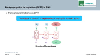
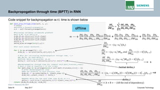
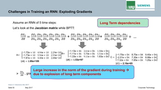
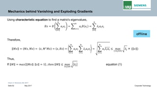
Backpropogation through time (BPTT) in RNN
The output at time t=3 is dependent on the inputs from t=3 to t=1
𝜕𝜕𝐸𝐸
𝜕𝜕θ
= �
1≤𝑡𝑡≤3
𝜕𝜕𝐸𝐸𝑡𝑡
𝜕𝜕θ
𝜕𝜕𝐸𝐸3
𝜕𝜕Wℎℎ
=
𝜕𝜕𝐸𝐸3
𝜕𝜕ℎ3
𝜕𝜕ℎ3
𝜕𝜕Wℎℎ
Direction of Backward pass (via partial derivatives)
--- gradient flow ---
WhoWho
Who
Whh Whh
Writing gradients in a sum-of-products form
Since ℎ3 depends on ℎ2 𝐚𝐚𝐚𝐚𝐚𝐚 ℎ2 depends on ℎ1, therefore
𝜕𝜕𝐸𝐸3
𝜕𝜕Wℎℎ
= �
𝑘𝑘=1
3
𝜕𝜕𝐸𝐸3
𝜕𝜕ℎ3
𝜕𝜕ℎ3
𝜕𝜕ℎ𝑘𝑘
𝜕𝜕ℎ𝑘𝑘
𝜕𝜕Wℎℎ
𝜕𝜕ℎ𝑡𝑡
𝜕𝜕h𝑘𝑘
= �
𝑡𝑡≥𝑖𝑖>𝑘𝑘
𝜕𝜕ℎ𝑖𝑖
𝜕𝜕ℎ𝑖𝑖−1
= �
𝑡𝑡≥𝑖𝑖>𝑘𝑘
Wℎℎ
𝑇𝑇
𝑑𝑑𝑑𝑑𝑑𝑑𝑑𝑑[𝑔𝑔′(ℎ𝑖𝑖−1)]
Weight matrix
Derivative of activation function
𝜕𝜕ℎ3
𝜕𝜕h1
=
𝜕𝜕ℎ3
𝜕𝜕ℎ2
𝜕𝜕ℎ2
𝜕𝜕ℎ1
e.g.,
𝜕𝜕𝐸𝐸𝑡𝑡
𝜕𝜕Wℎℎ
= �
1≤𝑘𝑘≤𝑡𝑡
𝜕𝜕𝐸𝐸𝑡𝑡
𝜕𝜕ℎ𝑡𝑡
𝜕𝜕ℎ𝑡𝑡
𝜕𝜕ℎ𝑘𝑘
𝜕𝜕ℎ𝑘𝑘
𝜕𝜕Wℎℎ
In general,
Jacobian matrix
𝝏𝝏𝒉𝒉𝒕𝒕
𝝏𝝏𝒉𝒉𝒌𝒌
Transport error in time from step t back to step k

41. Intern © Siemens AG 2017
May 2017Seite 41 Corporate Technology
Direction of Backward pass (via partial derivatives)
--- gradient flow ---
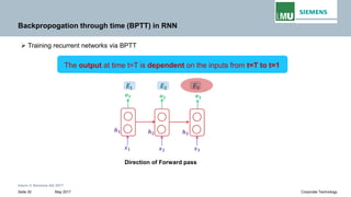
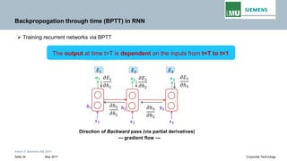
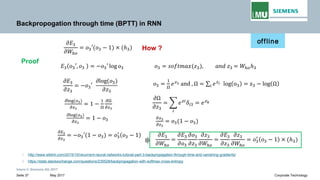
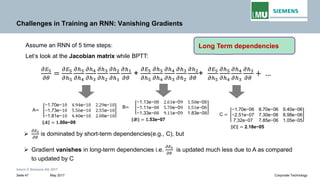
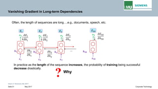
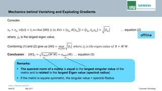
Backpropogation through time (BPTT) in RNN
The output at time t=3 is dependent on the inputs from t=3 to t=1
𝜕𝜕𝐸𝐸
𝜕𝜕θ
= �
1≤𝑡𝑡≤3
𝜕𝜕𝐸𝐸𝑡𝑡
𝜕𝜕θ
𝜕𝜕𝐸𝐸3
𝜕𝜕Wℎℎ
=
𝜕𝜕𝐸𝐸3
𝜕𝜕ℎ3
𝜕𝜕ℎ3
𝜕𝜕Wℎℎ
𝒐𝒐𝟐𝟐 𝒐𝒐𝟑𝟑
𝒐𝒐𝟏𝟏
𝐸𝐸1 𝐸𝐸2 𝐸𝐸3
𝒙𝒙𝟏𝟏 𝒙𝒙𝟐𝟐 𝒙𝒙𝟑𝟑
𝒉𝒉𝟏𝟏 𝒉𝒉𝟐𝟐 𝒉𝒉𝟑𝟑
𝜕𝜕𝐸𝐸3
𝜕𝜕ℎ3
𝜕𝜕𝐸𝐸2
𝜕𝜕ℎ2
𝜕𝜕𝐸𝐸1
𝜕𝜕ℎ1
𝜕𝜕ℎ2
𝜕𝜕ℎ1
𝜕𝜕ℎ3
𝜕𝜕ℎ2
WhoWho
Who
Whh Whh
Writing gradients in a sum-of-products form
Since ℎ3 depends on ℎ2 𝐚𝐚𝐚𝐚𝐚𝐚 ℎ2 depends on ℎ1, therefore
𝜕𝜕𝐸𝐸3
𝜕𝜕Wℎℎ
= �
𝑘𝑘=1
3
𝜕𝜕𝐸𝐸3
𝜕𝜕ℎ3
𝜕𝜕ℎ3
𝜕𝜕ℎ𝑘𝑘
𝜕𝜕ℎ𝑘𝑘
𝜕𝜕Wℎℎ
𝜕𝜕𝐸𝐸𝑡𝑡
𝜕𝜕Wℎℎ
= �
1≤𝑘𝑘≤𝑡𝑡
𝜕𝜕𝐸𝐸3
𝜕𝜕ℎ𝑡𝑡
𝜕𝜕ℎ𝑡𝑡
𝜕𝜕ℎ𝑘𝑘
𝜕𝜕ℎ𝑘𝑘
𝜕𝜕Wℎℎ
𝜕𝜕ℎ𝑡𝑡
𝜕𝜕h𝑘𝑘
= �
𝑡𝑡≥𝑖𝑖>𝑘𝑘
𝜕𝜕ℎ𝑖𝑖
𝜕𝜕ℎ𝑖𝑖−1
= �
𝑡𝑡≥𝑖𝑖>𝑘𝑘
Wℎℎ
𝑇𝑇
𝑑𝑑𝑑𝑑𝑑𝑑𝑑𝑑[𝑔𝑔′(ℎ𝑖𝑖−1)]
Jacobian matrix
𝝏𝝏𝒉𝒉𝒕𝒕
𝝏𝝏𝒉𝒉𝒌𝒌
Transport error in time from step t back to step k
Repeated matrix multiplications leads to vanishing and exploding gradients
𝜕𝜕ℎ3
𝜕𝜕h1
=
𝜕𝜕ℎ3
𝜕𝜕ℎ2
𝜕𝜕ℎ2
𝜕𝜕ℎ1
e.g.,

42. Intern © Siemens AG 2017
May 2017Seite 42 Corporate Technology
BPTT: Gradient Flow
𝒙𝒙𝟐𝟐 𝒙𝒙𝟑𝟑
𝒐𝒐𝟐𝟐 𝒐𝒐𝟑𝟑
𝒙𝒙𝟏𝟏
𝒐𝒐𝟏𝟏
𝑾𝑾𝒉𝒉𝒉𝒉 𝑾𝑾𝒉𝒉𝒉𝒉
𝐸𝐸1 𝐸𝐸2 𝐸𝐸3
𝒉𝒉𝟐𝟐
𝜕𝜕𝐸𝐸3
𝜕𝜕Wℎℎ
= �
𝑘𝑘=1
3
𝜕𝜕𝐸𝐸3
𝜕𝜕ℎ3
𝜕𝜕ℎ3
𝜕𝜕ℎ𝑘𝑘
𝜕𝜕ℎ𝑘𝑘
𝜕𝜕Wℎℎ
=
𝜕𝜕𝐸𝐸3
𝜕𝜕𝑜𝑜3
𝜕𝜕𝑜𝑜3
𝜕𝜕ℎ3
𝜕𝜕ℎ3
𝜕𝜕ℎ2
𝜕𝜕ℎ2
𝜕𝜕ℎ1
𝜕𝜕ℎ1
𝜕𝜕𝑊𝑊ℎℎ
+
𝜕𝜕𝐸𝐸3
𝜕𝜕𝑜𝑜3
𝜕𝜕𝑜𝑜3
𝜕𝜕ℎ3
𝜕𝜕ℎ3
𝜕𝜕ℎ2
𝜕𝜕ℎ2
𝜕𝜕𝑊𝑊ℎℎ
+
𝜕𝜕𝐸𝐸3
𝜕𝜕𝑜𝑜3
𝜕𝜕𝑜𝑜3
𝜕𝜕ℎ3
𝜕𝜕ℎ3
𝜕𝜕ℎ3
𝜕𝜕ℎ3
𝜕𝜕𝑊𝑊ℎℎ 𝜕𝜕ℎ2
𝜕𝜕ℎ1
𝜕𝜕ℎ3
𝜕𝜕ℎ2
𝒉𝒉𝟏𝟏 𝒉𝒉𝟑𝟑

43. Intern © Siemens AG 2017
May 2017Seite 43 Corporate Technology
Backpropogation through time (BPTT) in RNN
Code snippet for forward-propagation is shown below (Before going for BPTT code) offline
https://cs224d.stanford.edu/lectures/CS224d-Lecture8.pdf

44. Intern © Siemens AG 2017
May 2017Seite 44 Corporate Technology
Backpropogation through time (BPTT) in RNN
Code snippet for backpropagation w.r.t. time is shown below
= ⋯ +
𝜕𝜕𝐸𝐸𝑡𝑡
𝜕𝜕𝑜𝑜𝑡𝑡
𝜕𝜕𝑜𝑜𝑡𝑡
𝜕𝜕ℎ𝑡𝑡
𝜕𝜕ℎ𝑡𝑡
𝜕𝜕ℎ𝑡𝑡−1
𝜕𝜕ℎ𝑡𝑡−1
𝜕𝜕ℎ𝑡𝑡−2
𝜕𝜕ℎ𝑡𝑡−2
𝜕𝜕𝑊𝑊ℎℎ
+
𝜕𝜕𝐸𝐸𝑡𝑡
𝜕𝜕𝑜𝑜𝑡𝑡
𝜕𝜕𝑜𝑜𝑡𝑡
𝜕𝜕ℎ𝑡𝑡
𝜕𝜕ℎ𝑡𝑡
𝜕𝜕ℎ𝑡𝑡−1
𝜕𝜕ℎ𝑡𝑡−1
𝜕𝜕𝑊𝑊ℎℎ
+
𝜕𝜕𝐸𝐸𝑡𝑡
𝜕𝜕𝑜𝑜𝑡𝑡
𝜕𝜕𝑜𝑜𝑡𝑡
𝜕𝜕ℎ𝑡𝑡
𝜕𝜕ℎ𝑡𝑡
𝜕𝜕𝑊𝑊ℎℎ
offline
𝝏𝝏𝑬𝑬𝒕𝒕
𝝏𝝏𝑾𝑾𝒉𝒉𝒉𝒉
= �
𝒌𝒌=𝟏𝟏
𝒕𝒕
𝝏𝝏𝑬𝑬𝒕𝒕
𝝏𝝏𝒉𝒉𝒕𝒕
𝝏𝝏𝒉𝒉𝒕𝒕
𝝏𝝏𝒉𝒉𝒌𝒌
𝝏𝝏𝒉𝒉𝒌𝒌
𝝏𝝏𝑾𝑾𝒉𝒉𝒉𝒉
𝜕𝜕𝐸𝐸𝑡𝑡
𝜕𝜕ℎ𝑡𝑡
= −(𝑜𝑜𝑡𝑡−𝑜𝑜𝑡𝑡′)𝑊𝑊ℎ𝑜𝑜 𝑎𝑎𝑎𝑎𝑎𝑎
𝜕𝜕ℎ𝑡𝑡
𝜕𝜕𝑊𝑊ℎℎ
= (1 − ℎ𝑡𝑡
2
)(ℎ𝑡𝑡−1)
𝜕𝜕𝐸𝐸
𝜕𝜕ℎ𝑡𝑡
𝜕𝜕ℎ𝑡𝑡
𝜕𝜕𝑊𝑊ℎℎ
= −(𝑜𝑜𝑡𝑡−𝑜𝑜𝑡𝑡′)𝑊𝑊ℎ𝑜𝑜(1 − ℎ𝑡𝑡
2
)(ℎ𝑡𝑡−1)
𝑰𝑰𝑰𝑰𝑰𝑰𝑰𝑰𝑰𝑰 𝑰𝑰𝑰𝑰 𝒅𝒅𝒅𝒅𝒅𝒅𝒅𝒅𝒅𝒅_𝒕𝒕
𝜕𝜕𝐸𝐸𝑡𝑡
𝜕𝜕𝑊𝑊ℎ𝑜𝑜
= −(𝑜𝑜𝑡𝑡−𝑜𝑜𝑡𝑡′)(ℎ𝑡𝑡)
𝜕𝜕𝐸𝐸𝑡𝑡
𝜕𝜕𝑜𝑜𝑡𝑡
𝜕𝜕𝑜𝑜𝑡𝑡
𝜕𝜕ℎ𝑡𝑡
𝜕𝜕ℎ𝑡𝑡
𝜕𝜕ℎ𝑡𝑡−1
𝜕𝜕ℎ𝑡𝑡−1
𝜕𝜕𝑊𝑊ℎℎ
= − 𝑜𝑜𝑡𝑡 − 𝑜𝑜𝑡𝑡
′
𝑊𝑊ℎ𝑜𝑜 1 − ℎ𝑡𝑡
2
(𝑊𝑊ℎℎ)(1 − ℎ𝑡𝑡−1
2
)(ℎ𝑡𝑡−2)
𝒅𝒅𝒅𝒅𝒅𝒅𝒅𝒅𝒅𝒅_𝒕𝒕
𝐀𝐀
𝑩𝑩
𝜕𝜕𝐸𝐸
𝜕𝜕𝑊𝑊ℎℎ
= A + B + ⋯ (till the end of dependency)

45. Intern © Siemens AG 2017
May 2017Seite 45 Corporate Technology
Break (10 minutes)

46. Intern © Siemens AG 2017
May 2017Seite 46 Corporate Technology
Challenges in Training an RNN: Vanishing Gradients
Short Term Dependencies
 need recent information to perform the present task.
For example in a language model, predict the next word based on the previous ones.
“the clouds are in the ?”  ‘sky’
 Easier to predict ‘sky’ given the context, i.e., short term dependency  (vanilla) RNN Good so far.
 Consider longer word sequence “I grew up in France…........…………………… I speak fluent French.”
 Recent information suggests that the next word is probably the name of a language, but if we want to
narrow down which language, we need the context of France, from further back.
 As the gap increases  practically difficult for RNN to learn from the past information
Long Term Dependencies
http://colah.github.io/posts/2015-08-Understanding-LSTMs/

47. Intern © Siemens AG 2017
May 2017Seite 47 Corporate Technology
Challenges in Training an RNN: Vanishing Gradients
Assume an RNN of 5 time steps:
Let‘s look at the Jacobian matrix while BPTT:
𝜕𝜕𝐸𝐸5
𝜕𝜕𝜃𝜃
=
𝜕𝜕𝐸𝐸5
𝜕𝜕ℎ5
𝜕𝜕ℎ5
𝜕𝜕ℎ4
𝜕𝜕ℎ4
𝜕𝜕ℎ3
𝜕𝜕ℎ3
𝜕𝜕ℎ2
𝜕𝜕ℎ2
𝜕𝜕ℎ1
𝜕𝜕ℎ1
𝜕𝜕𝜃𝜃
+
𝜕𝜕𝐸𝐸5
𝜕𝜕ℎ5
𝜕𝜕ℎ5
𝜕𝜕ℎ4
𝜕𝜕ℎ4
𝜕𝜕ℎ3
𝜕𝜕ℎ3
𝜕𝜕ℎ2
𝜕𝜕ℎ2
𝜕𝜕𝜃𝜃
+
𝜕𝜕𝐸𝐸5
𝜕𝜕ℎ5
𝜕𝜕ℎ5
𝜕𝜕ℎ4
𝜕𝜕ℎ4
𝜕𝜕ℎ3
𝜕𝜕ℎ3
𝜕𝜕𝜃𝜃
+ …
−1.70e−06 8.70e−06 9.40e−06
−2.51e−07 7.30e−06 8.98e−06
7.32e−07 7.85e−06 1.05e−05
C =
𝑪𝑪 = 2.18e−05
−1.13e−08 2.61e−09 1.50e−08
−1.11e−08 5.70e−09 1.51e−08
−1.33e−08 9.11e−09 1.83e−08
B=
𝑩𝑩 = 1.53e−07
−1.70e−10 4.94e−10 2.29e−10
−1.73e−10 5.56e−10 2.55e−10
−1.81e−10 4.40e−10 2.08e−10
A=
𝑨𝑨 = 1.00e−09

𝜕𝜕𝐸𝐸5
𝜕𝜕𝜕𝜕
is dominated by short-term dependencies(e.g., C), but
 Gradient vanishes in long-term dependencies i.e.
𝜕𝜕𝐸𝐸5
𝜕𝜕𝜕𝜕
is updated much less due to A as compared
to updated by C
Long Term dependencies

48. Intern © Siemens AG 2017
May 2017Seite 48 Corporate Technology
Challenges in Training an RNN: Vanishing Gradients
Assume an RNN of 5 time steps:
Let‘s look at the Jacobian matrix while BPTT:
𝜕𝜕𝐸𝐸5
𝜕𝜕𝜃𝜃
=
𝜕𝜕𝐸𝐸5
𝜕𝜕ℎ5
𝜕𝜕ℎ5
𝜕𝜕ℎ4
𝜕𝜕ℎ4
𝜕𝜕ℎ3
𝜕𝜕ℎ3
𝜕𝜕ℎ2
𝜕𝜕ℎ2
𝜕𝜕ℎ1
𝜕𝜕ℎ1
𝜕𝜕𝜃𝜃
+
𝜕𝜕𝐸𝐸5
𝜕𝜕ℎ5
𝜕𝜕ℎ5
𝜕𝜕ℎ4
𝜕𝜕ℎ4
𝜕𝜕ℎ3
𝜕𝜕ℎ3
𝜕𝜕ℎ2
𝜕𝜕ℎ2
𝜕𝜕𝜃𝜃
+
𝜕𝜕𝐸𝐸5
𝜕𝜕ℎ5
𝜕𝜕ℎ5
𝜕𝜕ℎ4
𝜕𝜕ℎ4
𝜕𝜕ℎ3
𝜕𝜕ℎ3
𝜕𝜕𝜃𝜃
+ …
−1.70e−06 8.70e−06 9.40e−06
−2.51e−07 7.30e−06 8.98e−06
7.32e−07 7.85e−06 1.05e−05
C =
𝑪𝑪 = 2.18e−05
−1.13e−08 2.61e−09 1.50e−08
−1.11e−08 5.70e−09 1.51e−08
−1.33e−08 9.11e−09 1.83e−08
B=
𝑩𝑩 = 1.53e−07
−1.70e−10 4.94e−10 2.29e−10
−1.73e−10 5.56e−10 2.55e−10
−1.81e−10 4.40e−10 2.08e−10
A=
𝑨𝑨 = 1.00e−09

𝜕𝜕𝐸𝐸5
𝜕𝜕𝜕𝜕
is dominated by short-term dependencies(e.g., C), but
 Gradient vanishes in long-term dependencies i.e.
𝜕𝜕𝐸𝐸5
𝜕𝜕𝜕𝜕
is updated much less due to A as compared
to updated by C
Long Term Components goes exponentially fast to norm 0
 no correlation between temporally distant events
Long Term dependencies

49. Intern © Siemens AG 2017
May 2017Seite 49 Corporate Technology
Challenges in Training an RNN: Exploding Gradients
Assume an RNN of 5 time steps:
Let‘s look at the Jacobian matrix while BPTT:
𝜕𝜕𝐸𝐸5
𝜕𝜕𝜃𝜃
=
𝜕𝜕𝐸𝐸5
𝜕𝜕ℎ5
𝜕𝜕ℎ5
𝜕𝜕ℎ4
𝜕𝜕ℎ4
𝜕𝜕ℎ3
𝜕𝜕ℎ3
𝜕𝜕ℎ2
𝜕𝜕ℎ2
𝜕𝜕ℎ1
𝜕𝜕ℎ1
𝜕𝜕𝜃𝜃
+
𝜕𝜕𝐸𝐸5
𝜕𝜕ℎ5
𝜕𝜕ℎ5
𝜕𝜕ℎ4
𝜕𝜕ℎ4
𝜕𝜕ℎ3
𝜕𝜕ℎ3
𝜕𝜕ℎ2
𝜕𝜕ℎ2
𝜕𝜕𝜃𝜃
+
𝜕𝜕𝐸𝐸5
𝜕𝜕ℎ5
𝜕𝜕ℎ5
𝜕𝜕ℎ4
𝜕𝜕ℎ4
𝜕𝜕ℎ3
𝜕𝜕ℎ3
𝜕𝜕𝜃𝜃
+ …
−1.70e + 06 8.70e + 06 9.40e + 06
−2.51e + 07 7.30e + 06 8.98e + 06
7.32e + 07 7.85e + 06 1.05e + 05
C =
𝑪𝑪 = 2.18e+105
−1.13e + 08 2.61e + 09 1.50e + 08
−1.11e + 08 5.70e + 09 1.51e + 08
−1.33e + 08 9.11e + 09 1.83e + 08
B=
𝑩𝑩 = 1.53e+107
−1.70e + 10 4.94e + 10 2.29e−10
−1.73e + 10 5.56e + 10 2.55e−10
−1.81e + 10 4.40e + 10 2.08e−10
A=
𝑨𝑨 = 1.00e+109

𝜕𝜕𝐸𝐸5
𝜕𝜕𝜕𝜕
, gradient explodes, i.e., NaN due to very large numbers
Long Term dependencies

50. Intern © Siemens AG 2017
May 2017Seite 50 Corporate Technology
Challenges in Training an RNN: Exploding Gradients
Assume an RNN of 5 time steps:
Let‘s look at the Jacobian matrix while BPTT:
𝜕𝜕𝐸𝐸5
𝜕𝜕𝜃𝜃
=
𝜕𝜕𝐸𝐸5
𝜕𝜕ℎ5
𝜕𝜕ℎ5
𝜕𝜕ℎ4
𝜕𝜕ℎ4
𝜕𝜕ℎ3
𝜕𝜕ℎ3
𝜕𝜕ℎ2
𝜕𝜕ℎ2
𝜕𝜕ℎ1
𝜕𝜕ℎ1
𝜕𝜕𝜃𝜃
+
𝜕𝜕𝐸𝐸5
𝜕𝜕ℎ5
𝜕𝜕ℎ5
𝜕𝜕ℎ4
𝜕𝜕ℎ4
𝜕𝜕ℎ3
𝜕𝜕ℎ3
𝜕𝜕ℎ2
𝜕𝜕ℎ2
𝜕𝜕𝜃𝜃
+
𝜕𝜕𝐸𝐸5
𝜕𝜕ℎ5
𝜕𝜕ℎ5
𝜕𝜕ℎ4
𝜕𝜕ℎ4
𝜕𝜕ℎ3
𝜕𝜕ℎ3
𝜕𝜕𝜃𝜃
+ …
−1.70e + 04 8.70e + 04 9.40e + 04
−2.51e + 04 7.30e + 04 8.98e + 04
7.32e + 04 7.85e + 04 1.05e + 04
C =
𝑪𝑪 = 2.18e+85
−1.13e + 06 2.61e + 06 1.50e + 06
−1.11e + 06 5.70e + 06 1.51e + 06
−1.33e + 06 9.11e + 06 1.83e + 06
B=
𝑩𝑩 = 1.53e+97
−1.70e + 10 4.94e + 10 2.29e−10
−1.73e + 10 5.56e + 10 2.55e−10
−1.81e + 10 4.40e + 10 2.08e−10
A=
𝑨𝑨 = 1.00e+109

𝜕𝜕𝐸𝐸5
𝜕𝜕𝜕𝜕
, gradient explodes, i.e., NaN due to very large numbers
Large increase in the norm of the gradient during training 
due to explosion of long term components
Long Term dependencies

51. Intern © Siemens AG 2017
May 2017Seite 51 Corporate Technology
Vanishing Gradient in Long-term Dependencies
Often, the length of sequences are long….e.g., documents, speech, etc.
𝒐𝒐𝟐𝟐 𝒐𝒐𝟑𝟑
𝒐𝒐𝟏𝟏
𝐸𝐸1 𝐸𝐸2 𝐸𝐸3
𝒙𝒙𝟏𝟏 𝒙𝒙𝟐𝟐 𝒙𝒙𝟑𝟑
𝒉𝒉𝟏𝟏 𝒉𝒉𝟐𝟐 𝒉𝒉𝟑𝟑
𝜕𝜕𝐸𝐸3
𝜕𝜕ℎ3
𝜕𝜕𝐸𝐸2
𝜕𝜕ℎ2
𝜕𝜕𝐸𝐸1
𝜕𝜕ℎ1
𝜕𝜕ℎ2
𝜕𝜕ℎ1
𝜕𝜕ℎ3
𝜕𝜕ℎ2
𝒐𝒐𝟑𝟑
𝐸𝐸50
𝒙𝒙𝟓𝟓𝟓𝟓
𝒉𝒉𝟓𝟓𝟓𝟓
𝜕𝜕𝐸𝐸50
𝜕𝜕ℎ50
…
In practice as the length of the sequence increases, the probability of training being successful
decrease drastically.
Why

52. Intern © Siemens AG 2017
May 2017Seite 53 Corporate Technology
Vanishing Gradient in Long-term Dependencies
Why
Let us look at the recurrent part of our RNN equation:
ℎ𝑡𝑡 = 𝑊𝑊ℎℎf(ℎt−1) + some other terms
ℎ𝑡𝑡 = 𝑊𝑊ℎℎℎ0 + some other terms
ℎ𝑡𝑡 = 𝑔𝑔𝑊𝑊 ℎ𝑡𝑡−1, 𝑥𝑥𝑡𝑡
ℎ𝑡𝑡 = tanh(𝑊𝑊ℎℎ ℎ𝑡𝑡−1 + 𝑊𝑊𝑥𝑥ℎ 𝑥𝑥𝑡𝑡)
𝑜𝑜𝑡𝑡 = 𝑠𝑠𝑠𝑠𝑠𝑠𝑠𝑠𝑠𝑠𝑠𝑠𝑠𝑠(𝑊𝑊ℎ𝑜𝑜ℎ𝑡𝑡)
tanh Expansion

53. Intern © Siemens AG 2017
May 2017Seite 54 Corporate Technology
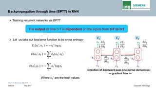
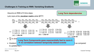
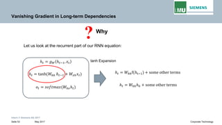
Vanishing Gradient in Long-term Dependencies
𝜕𝜕𝐸𝐸
𝜕𝜕θ
= �
1≤𝑡𝑡≤3
𝜕𝜕𝐸𝐸𝑡𝑡
𝜕𝜕θ
𝜕𝜕𝐸𝐸3
𝜕𝜕Wℎℎ
=
𝜕𝜕𝐸𝐸3
𝜕𝜕ℎ3
𝜕𝜕ℎ3
𝜕𝜕Wℎℎ
Direction of Backward pass (via partial derivatives)
--- gradient flow ---
𝒐𝒐𝟐𝟐 𝒐𝒐𝟑𝟑
𝒐𝒐𝟏𝟏
𝐸𝐸1 𝐸𝐸2 𝐸𝐸3
𝒙𝒙𝟏𝟏 𝒙𝒙𝟐𝟐 𝒙𝒙𝟑𝟑
𝒉𝒉𝟏𝟏 𝒉𝒉𝟐𝟐 𝒉𝒉𝟑𝟑
𝜕𝜕𝐸𝐸3
𝜕𝜕ℎ3
𝜕𝜕𝐸𝐸2
𝜕𝜕ℎ2
𝜕𝜕𝐸𝐸1
𝜕𝜕ℎ1
𝜕𝜕ℎ2
𝜕𝜕ℎ1
𝜕𝜕ℎ3
𝜕𝜕ℎ2
WhoWho
Who
Whh Whh
Writing gradients in a sum-of-products form
Since ℎ3 depends on ℎ2 𝐚𝐚𝐚𝐚𝐚𝐚 ℎ2 depends on ℎ1, therefore
𝜕𝜕𝐸𝐸3
𝜕𝜕Wℎℎ
= �
𝑘𝑘=0
3
𝜕𝜕𝐸𝐸3
𝜕𝜕ℎ3
𝜕𝜕ℎ3
𝜕𝜕ℎ𝑘𝑘
𝜕𝜕ℎ𝑘𝑘
𝜕𝜕Wℎℎ
𝜕𝜕𝐸𝐸𝑡𝑡
𝜕𝜕Wℎℎ
= �
1≤𝑘𝑘≤𝑡𝑡
𝜕𝜕𝐸𝐸𝑡𝑡
𝜕𝜕ℎ𝑡𝑡
𝜕𝜕ℎ𝑡𝑡
𝜕𝜕ℎ𝑘𝑘
𝜕𝜕ℎ𝑘𝑘
𝜕𝜕Wℎℎ
𝜕𝜕ℎ𝑡𝑡
𝜕𝜕h𝑘𝑘
= �
𝑡𝑡≥𝑖𝑖>𝑘𝑘
𝜕𝜕ℎ𝑖𝑖
𝜕𝜕ℎ𝑖𝑖−1
= �
𝑡𝑡≥𝑖𝑖>𝑘𝑘
Wℎℎ
𝑇𝑇
𝑑𝑑𝑑𝑑𝑑𝑑𝑑𝑑[𝑔𝑔′(ℎ𝑖𝑖−1)]
𝜕𝜕ℎ3
𝜕𝜕h1
=
𝜕𝜕ℎ3
𝜕𝜕ℎ2
𝜕𝜕ℎ2
𝜕𝜕ℎ1
Jacobian matrix
𝝏𝝏𝒉𝒉𝒕𝒕
𝝏𝝏𝒉𝒉𝒌𝒌
Transport error in time from step t back to step k
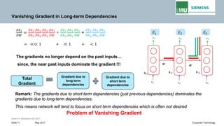
This term is the product of Jacobian matrix .
𝒉𝒉𝒕𝒕 = 𝑾𝑾𝒉𝒉𝒉𝒉 𝐟𝐟(𝒉𝒉𝐭𝐭− 𝟏𝟏) + 𝐬𝐬𝐬𝐬𝐬𝐬𝐬𝐬 𝐭𝐭𝐭𝐭𝐭𝐭𝐭𝐭𝐭𝐭
e.g.,
In general,

54. Intern © Siemens AG 2017
May 2017Seite 55 Corporate Technology
Vanishing Gradient in Long-term Dependencies
𝜕𝜕𝐸𝐸
𝜕𝜕θ
= �
1≤𝑡𝑡≤3
𝜕𝜕𝐸𝐸𝑡𝑡
𝜕𝜕θ
𝜕𝜕𝐸𝐸3
𝜕𝜕Wℎℎ
=
𝜕𝜕𝐸𝐸3
𝜕𝜕ℎ3
𝜕𝜕ℎ3
𝜕𝜕Wℎℎ
Direction of Backward pass (via partial derivatives)
--- gradient flow ---
𝒐𝒐𝟐𝟐 𝒐𝒐𝟑𝟑
𝒐𝒐𝟏𝟏
𝐸𝐸1 𝐸𝐸2 𝐸𝐸3
𝒙𝒙𝟏𝟏 𝒙𝒙𝟐𝟐 𝒙𝒙𝟑𝟑
𝒉𝒉𝟏𝟏 𝒉𝒉𝟐𝟐 𝒉𝒉𝟑𝟑
𝜕𝜕𝐸𝐸3
𝜕𝜕ℎ3
𝜕𝜕𝐸𝐸2
𝜕𝜕ℎ2
𝜕𝜕𝐸𝐸1
𝜕𝜕ℎ1
𝜕𝜕ℎ2
𝜕𝜕ℎ1
𝜕𝜕ℎ3
𝜕𝜕ℎ2
WhoWho
Who
Whh Whh
Writing gradients in a sum-of-products form
𝜕𝜕𝐸𝐸𝑡𝑡
𝜕𝜕Wℎℎ
= �
1≤𝑘𝑘≤𝑡𝑡
𝜕𝜕𝐸𝐸3
𝜕𝜕ℎ𝑡𝑡
𝜕𝜕ℎ𝑡𝑡
𝜕𝜕ℎ𝑘𝑘
𝜕𝜕ℎ𝑘𝑘
𝜕𝜕Wℎℎ
𝜕𝜕ℎ𝑡𝑡
𝜕𝜕h𝑘𝑘
= �
𝑡𝑡≥𝑖𝑖>𝑘𝑘
𝜕𝜕ℎ𝑖𝑖
𝜕𝜕ℎ𝑖𝑖−1
= �
𝑡𝑡≥𝑖𝑖>𝑘𝑘
Wℎℎ
𝑇𝑇
𝑑𝑑𝑑𝑑𝑑𝑑𝑑𝑑[𝑔𝑔′(ℎ𝑖𝑖−1)]
Jacobian matrix
𝝏𝝏𝒉𝒉𝒕𝒕
𝝏𝝏𝒉𝒉𝒌𝒌

55. Intern © Siemens AG 2017
May 2017Seite 56 Corporate Technology
Vanishing Gradient in Long-term Dependencies
𝜕𝜕𝐸𝐸
𝜕𝜕θ
= �
1≤𝑡𝑡≤3
𝜕𝜕𝐸𝐸𝑡𝑡
𝜕𝜕θ
𝜕𝜕𝐸𝐸3
𝜕𝜕Wℎℎ
=
𝜕𝜕𝐸𝐸3
𝜕𝜕ℎ3
𝜕𝜕ℎ3
𝜕𝜕Wℎℎ
Direction of Backward pass (via partial derivatives)
--- gradient flow ---
𝒐𝒐𝟐𝟐 𝒐𝒐𝟑𝟑
𝒐𝒐𝟏𝟏
𝐸𝐸1 𝐸𝐸2 𝐸𝐸3
𝒙𝒙𝟏𝟏 𝒙𝒙𝟐𝟐 𝒙𝒙𝟑𝟑
𝒉𝒉𝟏𝟏 𝒉𝒉𝟐𝟐 𝒉𝒉𝟑𝟑
𝜕𝜕𝐸𝐸3
𝜕𝜕ℎ3
𝜕𝜕𝐸𝐸2
𝜕𝜕ℎ2
𝜕𝜕𝐸𝐸1
𝜕𝜕ℎ1
𝜕𝜕ℎ2
𝜕𝜕ℎ1
𝜕𝜕ℎ3
𝜕𝜕ℎ2
WhoWho
Who
Whh Whh
Writing gradients in a sum-of-products form
𝜕𝜕𝐸𝐸𝑡𝑡
𝜕𝜕Wℎℎ
= �
1≤𝑘𝑘≤𝑡𝑡
𝜕𝜕𝐸𝐸3
𝜕𝜕ℎ𝑡𝑡
𝜕𝜕ℎ𝑡𝑡
𝜕𝜕ℎ𝑘𝑘
𝜕𝜕ℎ𝑘𝑘
𝜕𝜕Wℎℎ
𝜕𝜕ℎ𝑡𝑡
𝜕𝜕h𝑘𝑘
= �
𝑡𝑡≥𝑖𝑖>𝑘𝑘
𝜕𝜕ℎ𝑖𝑖
𝜕𝜕ℎ𝑖𝑖−1
= �
𝑡𝑡≥𝑖𝑖>𝑘𝑘
Wℎℎ
𝑇𝑇
𝑑𝑑𝑑𝑑𝑑𝑑𝑑𝑑[𝑔𝑔′(ℎ𝑖𝑖−1)]
Repeated matrix multiplications leads to vanishing gradients !!!

56. Intern © Siemens AG 2017
May 2017Seite 57 Corporate Technology
Mechanics behind Vanishing and Exploding Gradients
Direction of Backward pass (via partial derivatives)
--- gradient flow ---
𝒐𝒐𝟐𝟐 𝒐𝒐𝟑𝟑
𝒐𝒐𝟏𝟏
𝐸𝐸1 𝐸𝐸2 𝐸𝐸3
𝒙𝒙𝟏𝟏 𝒙𝒙𝟐𝟐 𝒙𝒙𝟑𝟑
𝒉𝒉𝟏𝟏 𝒉𝒉𝟐𝟐 𝒉𝒉𝟑𝟑
𝜕𝜕𝐸𝐸3
𝜕𝜕ℎ3
𝜕𝜕𝐸𝐸2
𝜕𝜕ℎ2
𝜕𝜕𝐸𝐸1
𝜕𝜕ℎ1
𝜕𝜕ℎ2
𝜕𝜕ℎ1
𝜕𝜕ℎ3
𝜕𝜕ℎ2
WhoWho
Who
Whh Whh
𝜕𝜕ℎ𝑡𝑡
𝜕𝜕h𝑘𝑘
= �
𝑡𝑡≥𝑖𝑖>𝑘𝑘
𝜕𝜕ℎ𝑖𝑖
𝜕𝜕ℎ𝑖𝑖−1
= �
𝑡𝑡≥𝑖𝑖>𝑘𝑘
Wℎℎ
𝑇𝑇
𝑑𝑑𝑑𝑑𝑑𝑑𝑑𝑑[𝑔𝑔′(ℎ𝑖𝑖−1)]
Consider identity activation function
If recurrent matrix Wℎℎ is a diagonalizable:
𝑾𝑾𝒉𝒉𝒉𝒉 = 𝑸𝑸−𝟏𝟏
∗ 𝜵𝜵 ∗ 𝑸𝑸
matrix composed of eigenvectors of Wℎℎ
diagonal matrix with eigenvalues placed on the diagonals
Using power iteration method, computing powers of Wℎℎ :
𝑾𝑾𝒉𝒉𝒉𝒉 = 𝑸𝑸−𝟏𝟏
∗ 𝜵𝜵 ∗ 𝑸𝑸
n n
Bengio et al, "On the difficulty of training recurrent neural networks." (2012)

57. Intern © Siemens AG 2017
May 2017Seite 58 Corporate Technology
Mechanics behind Vanishing and Exploding Gradients
Direction of Backward pass (via partial derivatives)
𝒐𝒐𝟐𝟐 𝒐𝒐𝟑𝟑
𝒐𝒐𝟏𝟏
𝐸𝐸1 𝐸𝐸2 𝐸𝐸3
𝒙𝒙𝟏𝟏 𝒙𝒙𝟐𝟐 𝒙𝒙𝟑𝟑
𝒉𝒉𝟏𝟏 𝒉𝒉𝟐𝟐 𝒉𝒉𝟑𝟑
𝜕𝜕𝐸𝐸3
𝜕𝜕ℎ3
𝜕𝜕𝐸𝐸2
𝜕𝜕ℎ2
𝜕𝜕𝐸𝐸1
𝜕𝜕ℎ1
𝜕𝜕ℎ2
𝜕𝜕ℎ1
𝜕𝜕ℎ3
𝜕𝜕ℎ2
WhoWho
Who
Whh Whh
𝜕𝜕ℎ𝑡𝑡
𝜕𝜕h𝑘𝑘
= �
𝑡𝑡≥𝑖𝑖>𝑘𝑘
𝜕𝜕ℎ𝑖𝑖
𝜕𝜕ℎ𝑖𝑖−1
= �
𝑡𝑡≥𝑖𝑖>𝑘𝑘
Wℎℎ
𝑇𝑇
𝑑𝑑𝑑𝑑𝑑𝑑𝑑𝑑[𝑔𝑔′(ℎ𝑖𝑖−1)]
Consider identity activation function
computing powers of Wℎℎ :
𝑾𝑾𝒉𝒉𝒉𝒉 = 𝑸𝑸−𝟏𝟏 ∗ 𝜵𝜵 ∗ 𝑸𝑸
n n
Bengio et al, "On the difficulty of training recurrent neural networks." (2012)
𝜵𝜵 =
- 0.618
1.618
0
0
𝜵𝜵 =
- 0.0081
122.99
0
0
10
Exploding gradients
Vanishing gradients
Eigen values on the diagonal

58. Intern © Siemens AG 2017
May 2017Seite 59 Corporate Technology
Mechanics behind Vanishing and Exploding Gradients
𝜕𝜕ℎ𝑡𝑡
𝜕𝜕h𝑘𝑘
= �
𝑡𝑡≥𝑖𝑖>𝑘𝑘
𝜕𝜕ℎ𝑖𝑖
𝜕𝜕ℎ𝑖𝑖−1
= �
𝑡𝑡≥𝑖𝑖>𝑘𝑘
Wℎℎ
𝑇𝑇
𝑑𝑑𝑑𝑑𝑑𝑑𝑑𝑑[𝑔𝑔′(ℎ𝑖𝑖−1)]
Consider identity activation function
computing powers of Wℎℎ :
𝑾𝑾𝒉𝒉𝒉𝒉 = 𝑸𝑸−𝟏𝟏 ∗ 𝜵𝜵 ∗ 𝑸𝑸
n n
Bengio et al, "On the difficulty of training recurrent neural networks." (2012)
𝜵𝜵 =
- 0.618
1.618
0
0
𝜵𝜵 =
- 0.0081
122.99
0
0
10
Exploding gradients
Vanishing gradients
Eigen values on the diagonal
Need for tight conditions
on eigen values
during training to prevent
gradients to vanish or explode

59. Intern © Siemens AG 2017
May 2017Seite 60 Corporate Technology
Mechanics behind Vanishing and Exploding Gradients
𝜕𝜕𝐸𝐸
𝜕𝜕θ
= �
1≤𝑡𝑡≤3
𝜕𝜕𝐸𝐸𝑡𝑡
𝜕𝜕θ
𝜕𝜕𝐸𝐸3
𝜕𝜕Wℎℎ
=
𝜕𝜕𝐸𝐸3
𝜕𝜕ℎ3
𝜕𝜕ℎ3
𝜕𝜕Wℎℎ
Direction of Backward pass (via partial derivatives)
--- gradient flow ---
𝒐𝒐𝟐𝟐 𝒐𝒐𝟑𝟑
𝒐𝒐𝟏𝟏
𝐸𝐸1 𝐸𝐸2 𝐸𝐸3
𝒙𝒙𝟏𝟏 𝒙𝒙𝟐𝟐 𝒙𝒙𝟑𝟑
𝒉𝒉𝟏𝟏 𝒉𝒉𝟐𝟐 𝒉𝒉𝟑𝟑
𝜕𝜕𝐸𝐸3
𝜕𝜕ℎ3
𝜕𝜕𝐸𝐸2
𝜕𝜕ℎ2
𝜕𝜕𝐸𝐸1
𝜕𝜕ℎ1
𝜕𝜕ℎ2
𝜕𝜕ℎ1
𝜕𝜕ℎ3
𝜕𝜕ℎ2
WhoWho
Who
Whh Whh
Writing gradients in a sum-of-products form
𝜕𝜕𝐸𝐸𝑡𝑡
𝜕𝜕Wℎℎ
= �
1≤𝑘𝑘≤𝑡𝑡
𝜕𝜕𝐸𝐸3
𝜕𝜕ℎ𝑡𝑡
𝜕𝜕ℎ𝑡𝑡
𝜕𝜕ℎ𝑘𝑘
𝜕𝜕ℎ𝑘𝑘
𝜕𝜕Wℎℎ
𝜕𝜕ℎ𝑡𝑡
𝜕𝜕h𝑘𝑘
= �
𝑡𝑡≥𝑖𝑖>𝑘𝑘
𝜕𝜕ℎ𝑖𝑖
𝜕𝜕ℎ𝑖𝑖−1
= �
𝑡𝑡≥𝑖𝑖>𝑘𝑘
Wℎℎ
𝑇𝑇
𝑑𝑑𝑑𝑑𝑑𝑑𝑑𝑑[𝑔𝑔′(ℎ𝑖𝑖−1)]
� �
𝜕𝜕ℎ𝑖𝑖
𝜕𝜕ℎ𝑖𝑖−1
≤ Wℎℎ
𝑇𝑇
𝑑𝑑𝑑𝑑𝑑𝑑𝑑𝑑 𝑔𝑔′ ℎ𝑖𝑖−1
Find Sufficient condition for when gradients vanish  compute an upper bound for
𝜕𝜕ℎ𝑡𝑡
𝜕𝜕ℎ𝑘𝑘
term
 find out an upper bound for the norm of the jacobian!

60. Intern © Siemens AG 2017
May 2017Seite 61 Corporate Technology
Mechanics behind Vanishing and Exploding Gradients
Lets find an upper bound for the term: 𝑾𝑾𝑻𝑻
𝒅𝒅𝒅𝒅𝒅𝒅𝒅𝒅 𝒈𝒈′
𝒉𝒉𝒊𝒊−𝟏𝟏
• Proof: 𝑀𝑀 2 = 𝜆𝜆 𝑚𝑚𝑚𝑚𝑚𝑚(𝑀𝑀∗ 𝑀𝑀) = 𝛾𝛾𝑚𝑚𝑚𝑚𝑚𝑚(M)
where the spectral norm 𝑀𝑀 2‖of a complex matrix 𝑀𝑀 is defined as 𝑚𝑚𝑚𝑚𝑚𝑚 𝑀𝑀𝑀𝑀 2: 𝑥𝑥 = 1
Put 𝐵𝐵 = 𝑀𝑀 ∗ 𝑀𝑀 which is a Hermitian matrix. As a linear transformation of Euclidean vector space 𝐸𝐸 is Hermite
iff there exists an orthonormal basis of 𝐸𝐸 consisting of all the eigenvectors of 𝐵𝐵
Let 𝜆𝜆1, 𝜆𝜆2, 𝜆𝜆3 … 𝜆𝜆𝑛𝑛 be the eigenvalues of 𝐵𝐵 and 𝑒𝑒1, 𝑒𝑒2 … … . 𝑒𝑒𝑛𝑛 be an orthonormal basis of 𝐸𝐸
Let 𝑥𝑥 = 𝑎𝑎1 𝑒𝑒1 + … … 𝑎𝑎𝑛𝑛 𝑒𝑒𝑛𝑛 (linear combination of eigen vectors)
The specttal norm of x:
𝑥𝑥 = ∑𝑖𝑖=1
𝑛𝑛
𝑎𝑎𝑖𝑖 𝑒𝑒𝑖𝑖 ∑𝑖𝑖=1
𝑛𝑛
𝑎𝑎𝑖𝑖 𝑒𝑒𝑖𝑖
1/2
= ∑𝑖𝑖=1
𝑛𝑛
𝑎𝑎𝑖𝑖
2
The norm of a matrix is equal to the largest singular value of the matrix and is
related to the largest Eigen value (spectral radius)
Property of matrix norm
offline

61. Intern © Siemens AG 2017
May 2017Seite 62 Corporate Technology
Mechanics behind Vanishing and Exploding Gradients
Using characteristic equation to find a matrix's eigenvalues,
𝐵𝐵𝐵𝐵 = 𝐵𝐵 �
𝑖𝑖=1
𝑛𝑛
𝑎𝑎𝑖𝑖 𝑒𝑒𝑖𝑖 = �
𝑖𝑖=1
𝑛𝑛
𝑎𝑎𝑖𝑖 𝐵𝐵 𝑒𝑒𝑖𝑖 = �
𝑖𝑖=1
𝑛𝑛
𝜆𝜆𝑖𝑖 𝑎𝑎𝑖𝑖 𝑒𝑒𝑖𝑖
Therefore,
𝑀𝑀𝑀𝑀 = 𝑀𝑀𝑀𝑀, 𝑀𝑀𝑀𝑀 = 𝑥𝑥, 𝑀𝑀∗
𝑀𝑀𝑀𝑀 = 𝑥𝑥, 𝐵𝐵𝐵𝐵 = �
𝑖𝑖=1
𝑛𝑛
𝑎𝑎𝑖𝑖 𝑒𝑒𝑖𝑖 �
𝑖𝑖=1
𝑛𝑛
𝜆𝜆𝑖𝑖 𝑎𝑎𝑖𝑖 𝑒𝑒𝑖𝑖 = �
𝑖𝑖=1
𝑛𝑛
𝑎𝑎𝑖𝑖 𝜆𝜆𝑖𝑖 𝑎𝑎𝑖𝑖 ≤ max
(1≤𝑗𝑗≤𝑛𝑛)
𝜆𝜆𝑗𝑗 × ( 𝑥𝑥 )
Thus,
If 𝑀𝑀 = 𝑚𝑚𝑚𝑚𝑚𝑚 𝑀𝑀𝑀𝑀 : 𝑥𝑥 = 1 , 𝑡𝑡ℎ𝑒𝑒𝑒𝑒 𝑀𝑀 ≤ max
1≤𝑗𝑗≤𝑛𝑛
𝜆𝜆𝑗𝑗 equation (1)
offline

62. Intern © Siemens AG 2017
May 2017Seite 63 Corporate Technology
Mechanics behind Vanishing and Exploding Gradients
Consider,
𝑥𝑥0 = 𝑒𝑒𝑗𝑗0
⇒ 𝑥𝑥 = 1, 𝑠𝑠𝑠𝑠 𝑡𝑡ℎ𝑎𝑎𝑎𝑎 𝑀𝑀 ≥ 𝑥𝑥, 𝐵𝐵𝐵𝐵 = 𝑒𝑒𝑗𝑗0
, 𝐵𝐵 𝑒𝑒𝑗𝑗0
= 𝑒𝑒𝑗𝑗0
, 𝜆𝜆𝑗𝑗0
𝑒𝑒𝑗𝑗0
= 𝜆𝜆𝑗𝑗0
… equation (2)
where, 𝑗𝑗0 is the largest eigen value.
Combining (1) and (2) give us 𝑀𝑀 = max
1≤𝑗𝑗≤𝑛𝑛
𝜆𝜆𝑗𝑗 𝑤𝑤ℎ𝑒𝑒𝑒𝑒𝑒𝑒, 𝜆𝜆𝑗𝑗 𝑖𝑖𝑖𝑖 𝑡𝑡ℎ𝑒𝑒 𝑒𝑒𝑒𝑒𝑒𝑒𝑒𝑒𝑒𝑒 𝑣𝑣𝑣𝑣𝑣𝑣𝑣𝑣𝑣𝑣 𝑜𝑜𝑜𝑜 𝐵𝐵 = 𝑀𝑀∗
𝑀𝑀
Conclusion : 𝑀𝑀 2 = 𝜆𝜆 𝑚𝑚𝑚𝑚𝑚𝑚(𝑀𝑀∗ 𝑀𝑀) = 𝛾𝛾𝑚𝑚𝑚𝑚𝑚𝑚(M) …. equation (3)
Remarks:
 The spectral norm of a matrix is equal to the largest singular value of the
matrix and is related to the largest Eigen value (spectral radius)
 If the matrix is square symmetric, the singular value = spectral Radius
offline

63. Intern © Siemens AG 2017
May 2017Seite 64 Corporate Technology
Mechanics behind Vanishing and Exploding Gradients
Let’s use these properties:
𝜕𝜕ℎ𝑡𝑡
𝜕𝜕h𝑘𝑘
= �
𝑡𝑡≥𝑖𝑖>𝑘𝑘
𝜕𝜕ℎ𝑖𝑖
𝜕𝜕ℎ𝑖𝑖−1
= �
𝑡𝑡≥𝑖𝑖>𝑘𝑘
Wℎℎ
𝑇𝑇
𝑑𝑑𝑑𝑑𝑑𝑑𝑑𝑑[𝑔𝑔′(ℎ𝑖𝑖−1)]
� �
𝜕𝜕ℎ𝑖𝑖
𝜕𝜕ℎ𝑖𝑖−1
≤ Wℎℎ
𝑇𝑇
𝑑𝑑𝑑𝑑𝑑𝑑𝑑𝑑 𝑔𝑔′
ℎ𝑖𝑖−1

64. Intern © Siemens AG 2017
May 2017Seite 65 Corporate Technology
Mechanics behind Vanishing and Exploding Gradients
Let’s use these properties:
𝜕𝜕ℎ𝑡𝑡
𝜕𝜕h𝑘𝑘
= �
𝑡𝑡≥𝑖𝑖>𝑘𝑘
𝜕𝜕ℎ𝑖𝑖
𝜕𝜕ℎ𝑖𝑖−1
= �
𝑡𝑡≥𝑖𝑖>𝑘𝑘
Wℎℎ
𝑇𝑇
𝑑𝑑𝑑𝑑𝑑𝑑𝑑𝑑[𝑔𝑔′(ℎ𝑖𝑖−1)]
� �
𝜕𝜕ℎ𝑖𝑖
𝜕𝜕ℎ𝑖𝑖−1
≤ Wℎℎ
𝑇𝑇
𝑑𝑑𝑑𝑑𝑑𝑑𝑑𝑑 𝑔𝑔′
ℎ𝑖𝑖−1
Gradient of the nonlinear function
(sigmoid or tanh) 𝑔𝑔′ ℎ𝑖𝑖−1 is bounded by
constant, .i.e., 𝑑𝑑𝑑𝑑𝑑𝑑𝑑𝑑 𝑔𝑔′ ℎ𝑖𝑖−1 ≤ 𝛾𝛾𝑔𝑔
an upper bound for the norm
of the gradient of activation
𝛾𝛾𝑔𝑔 = ¼ for sigmoid
𝛾𝛾𝑔𝑔 = 1 for tanh
constant

65. Intern © Siemens AG 2017
May 2017Seite 66 Corporate Technology
Mechanics behind Vanishing and Exploding Gradients
Let’s use these properties:
𝜕𝜕ℎ𝑡𝑡
𝜕𝜕h𝑘𝑘
= �
𝑡𝑡≥𝑖𝑖>𝑘𝑘
𝜕𝜕ℎ𝑖𝑖
𝜕𝜕ℎ𝑖𝑖−1
= �
𝑡𝑡≥𝑖𝑖>𝑘𝑘
Wℎℎ
𝑇𝑇
𝑑𝑑𝑑𝑑𝑑𝑑𝑑𝑑[𝑔𝑔′(ℎ𝑖𝑖−1)]
� �
𝜕𝜕ℎ𝑖𝑖
𝜕𝜕ℎ𝑖𝑖−1
≤ Wℎℎ
𝑇𝑇
𝑑𝑑𝑑𝑑𝑑𝑑𝑑𝑑 𝑔𝑔′
ℎ𝑖𝑖−1
Gradient of the nonlinear function
(sigmoid or tanh) 𝑔𝑔′ ℎ𝑖𝑖−1 is bounded by
constant, .i.e., 𝑑𝑑𝑑𝑑𝑑𝑑𝑑𝑑 𝑔𝑔′ ℎ𝑖𝑖−1 ≤ 𝛾𝛾𝑔𝑔
an upper bound for the norm
of the gradient of activation
𝛾𝛾𝑔𝑔 = ¼ for sigmoid
𝛾𝛾𝑔𝑔 = 1 for tanh
𝜸𝜸 𝑾𝑾 𝜸𝜸𝒈𝒈 = an upper bound for the norm of jacobian!
≤ 𝛾𝛾𝑊𝑊 𝛾𝛾𝑔𝑔
Largest Singular
value of 𝑾𝑾𝒉𝒉𝒉𝒉
constant

66. Intern © Siemens AG 2017
May 2017Seite 67 Corporate Technology
Mechanics behind Vanishing and Exploding Gradients
Let’s use these properties:
𝜕𝜕ℎ𝑡𝑡
𝜕𝜕h𝑘𝑘
= �
𝑡𝑡≥𝑖𝑖>𝑘𝑘
𝜕𝜕ℎ𝑖𝑖
𝜕𝜕ℎ𝑖𝑖−1
= �
𝑡𝑡≥𝑖𝑖>𝑘𝑘
Wℎℎ
𝑇𝑇
𝑑𝑑𝑑𝑑𝑑𝑑𝑑𝑑[𝑔𝑔′(ℎ𝑖𝑖−1)]
� �
𝜕𝜕ℎ𝑖𝑖
𝜕𝜕ℎ𝑖𝑖−1
≤ Wℎℎ
𝑇𝑇
𝑑𝑑𝑑𝑑𝑑𝑑𝑑𝑑 𝑔𝑔′
ℎ𝑖𝑖−1
Gradient of the nonlinear function
(sigmoid or tanh) 𝑔𝑔′ ℎ𝑖𝑖−1 is bounded by
constant, .i.e., 𝑑𝑑𝑑𝑑𝑑𝑑𝑑𝑑 𝑔𝑔′ ℎ𝑖𝑖−1 ≤ 𝛾𝛾𝑔𝑔
an upper bound for the norm
of the gradient of activation
𝜸𝜸 𝑾𝑾 𝜸𝜸𝒈𝒈 = an upper bound for the norm of jacobian!
≤ 𝛾𝛾𝑊𝑊 𝛾𝛾𝑔𝑔
Largest Singular
value of 𝑾𝑾𝒉𝒉𝒉𝒉
� �
𝜕𝜕ℎ3
𝜕𝜕ℎ𝑘𝑘
≤ 𝛾𝛾𝑊𝑊 𝛾𝛾𝑔𝑔
𝑡𝑡−𝑘𝑘

67. Intern © Siemens AG 2017
May 2017Seite 68 Corporate Technology
Mechanics behind Vanishing and Exploding Gradients
Let’s use these properties:
𝜕𝜕ℎ𝑡𝑡
𝜕𝜕h𝑘𝑘
= �
𝑡𝑡≥𝑖𝑖>𝑘𝑘
𝜕𝜕ℎ𝑖𝑖
𝜕𝜕ℎ𝑖𝑖−1
= �
𝑡𝑡≥𝑖𝑖>𝑘𝑘
Wℎℎ
𝑇𝑇
𝑑𝑑𝑑𝑑𝑑𝑑𝑑𝑑[𝑔𝑔′(ℎ𝑖𝑖−1)]
� �
𝜕𝜕ℎ𝑖𝑖
𝜕𝜕ℎ𝑖𝑖−1
≤ Wℎℎ
𝑇𝑇
𝑑𝑑𝑑𝑑𝑑𝑑𝑑𝑑 𝑔𝑔′
ℎ𝑖𝑖−1
𝜸𝜸 𝑾𝑾 𝜸𝜸𝒈𝒈 = an upper bound for the norm of jacobian!
≤ 𝛾𝛾𝑊𝑊 𝛾𝛾𝑔𝑔
Largest Singular
value of 𝑾𝑾𝒉𝒉𝒉𝒉
� �
𝜕𝜕ℎ3
𝜕𝜕ℎ𝑘𝑘
≤ 𝛾𝛾𝑊𝑊 𝛾𝛾𝑔𝑔
𝑡𝑡−𝑘𝑘
Sufficient Condition for Vanishing Gradient
As 𝛾𝛾𝑊𝑊 𝛾𝛾𝑔𝑔 < 1 and (t-k)∞ then long term
contributions go to 0 exponentially fast with t-k
(power iteration method).
Therefore,
sufficient condition for vanishing gradient to occur:
𝛾𝛾𝑊𝑊 < 1/𝛾𝛾𝑔𝑔
i.e. for sigmoid, 𝛾𝛾𝑊𝑊 < 4
i.e., for tanh, 𝛾𝛾𝑊𝑊 < 1

68. Intern © Siemens AG 2017
May 2017Seite 69 Corporate Technology
Mechanics behind Vanishing and Exploding Gradients
Let’s use these properties:
𝜕𝜕ℎ𝑡𝑡
𝜕𝜕h𝑘𝑘
= �
𝑡𝑡≥𝑖𝑖>𝑘𝑘
𝜕𝜕ℎ𝑖𝑖
𝜕𝜕ℎ𝑖𝑖−1
= �
𝑡𝑡≥𝑖𝑖>𝑘𝑘
Wℎℎ
𝑇𝑇
𝑑𝑑𝑑𝑑𝑑𝑑𝑑𝑑[𝑔𝑔′(ℎ𝑖𝑖−1)]
� �
𝜕𝜕ℎ𝑖𝑖
𝜕𝜕ℎ𝑖𝑖−1
≤ Wℎℎ
𝑇𝑇
𝑑𝑑𝑑𝑑𝑑𝑑𝑑𝑑 𝑔𝑔′
ℎ𝑖𝑖−1
𝜸𝜸 𝑾𝑾 𝜸𝜸𝒈𝒈 = an upper bound for the norm of jacobian!
≤ 𝛾𝛾𝑊𝑊 𝛾𝛾𝑔𝑔
Largest Singular
value of 𝑾𝑾𝒉𝒉𝒉𝒉
� �
𝜕𝜕ℎ3
𝜕𝜕ℎ𝑘𝑘
≤ 𝛾𝛾𝑊𝑊 𝛾𝛾𝑔𝑔
𝑡𝑡−𝑘𝑘
Necessary Condition for Exploding Gradient
As 𝛾𝛾𝑊𝑊 𝛾𝛾𝑔𝑔 > 1 and (t-k)∞ then gradient explodes!!!
Therefore,
Necessary condition for exploding gradient to occur:
𝛾𝛾𝑊𝑊> 1/𝛾𝛾𝑔𝑔
i.e. for sigmoid, 𝛾𝛾𝑊𝑊> 4
i.e., for tanh, 𝛾𝛾𝑊𝑊> 1

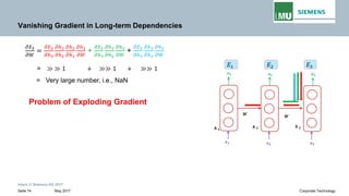
69. Intern © Siemens AG 2017
May 2017Seite 70 Corporate Technology
Vanishing Gradient in Long-term Dependencies
𝜕𝜕ℎ𝑡𝑡
𝜕𝜕h𝑘𝑘
= �
𝑡𝑡≥𝑖𝑖>𝑘𝑘
𝜕𝜕ℎ𝑖𝑖
𝜕𝜕ℎ𝑖𝑖−1
= �
𝑡𝑡≥𝑖𝑖>𝑘𝑘
Wℎℎ
𝑇𝑇
𝑑𝑑𝑑𝑑𝑑𝑑𝑑𝑑[𝑔𝑔′(ℎ𝑖𝑖−1)]
� �
𝜕𝜕ℎ𝑖𝑖
𝜕𝜕ℎ𝑖𝑖−1
≤ Wℎℎ
𝑇𝑇
𝑑𝑑𝑑𝑑𝑑𝑑𝑑𝑑 𝑔𝑔′ ℎ𝑖𝑖−1 ≤ 𝛾𝛾𝑊𝑊 𝛾𝛾𝑔𝑔
� �
𝜕𝜕ℎ3
𝜕𝜕ℎ𝑘𝑘
≤ 𝛾𝛾𝑊𝑊 𝛾𝛾𝑔𝑔
𝑡𝑡−𝑘𝑘
What have we concluded with the upper bound of derivative from recurrent step?
If we multiply the same term 𝛾𝛾𝑊𝑊 𝛾𝛾𝑔𝑔 < 1 again and again, the overall number becomes very
small(i.e almost equal to zero)
HOW ?
Repeated matrix multiplications leads to vanishing and exploding gradients

70. Intern © Siemens AG 2017
May 2017Seite 71 Corporate Technology
Vanishing Gradient in Long-term Dependencies
𝜕𝜕𝐸𝐸3
𝜕𝜕𝑊𝑊
=
𝜕𝜕𝐸𝐸3
𝜕𝜕ℎ3
𝜕𝜕ℎ3
𝜕𝜕ℎ2
𝜕𝜕ℎ2
𝜕𝜕ℎ1
𝜕𝜕ℎ1
𝜕𝜕𝑊𝑊
+
𝜕𝜕𝐸𝐸3
𝜕𝜕ℎ3
𝜕𝜕ℎ3
𝜕𝜕ℎ2
𝜕𝜕ℎ2
𝜕𝜕𝑊𝑊
+
𝜕𝜕𝐸𝐸3
𝜕𝜕ℎ3
𝜕𝜕ℎ3
𝜕𝜕ℎ3
𝜕𝜕ℎ3
𝜕𝜕𝑊𝑊
𝒙𝒙𝟐𝟐 𝒙𝒙𝟑𝟑
𝒐𝒐𝟐𝟐 𝒐𝒐𝟑𝟑
𝒙𝒙𝟏𝟏
𝒐𝒐𝟏𝟏
𝑾𝑾
𝑾𝑾
𝐸𝐸1 𝐸𝐸2 𝐸𝐸3
𝒉𝒉 𝟏𝟏
𝒉𝒉 𝟑𝟑𝒉𝒉 𝟐𝟐
≪≪ 1 ≪ 1 < 1+ +=
The gradients no longer depend on the past inputs…
since, the near past inputs dominate the gradient !!!
Problem of Vanishing Gradient
Total
Gradient
Gradient due to
long term
dependencies
Gradient due to
short term
dependencies
Remark: The gradients due to short term dependencies (just previous dependencies) dominates the
gradients due to long-term dependencies.
This means network will tend to focus on short term dependencies which is often not desired

71. Intern © Siemens AG 2017
May 2017Seite 72 Corporate Technology
Vanishing Gradient in Long-term Dependencies
𝜕𝜕𝐸𝐸3
𝜕𝜕𝑊𝑊
=
𝜕𝜕𝐸𝐸3
𝜕𝜕ℎ3
𝜕𝜕ℎ3
𝜕𝜕ℎ2
𝜕𝜕ℎ2
𝜕𝜕ℎ1
𝜕𝜕ℎ1
𝜕𝜕𝑊𝑊
+
𝜕𝜕𝐸𝐸3
𝜕𝜕ℎ3
𝜕𝜕ℎ3
𝜕𝜕ℎ2
𝜕𝜕ℎ2
𝜕𝜕𝑊𝑊
+
𝜕𝜕𝐸𝐸3
𝜕𝜕ℎ3
𝜕𝜕ℎ3
𝜕𝜕ℎ3
𝜕𝜕ℎ3
𝜕𝜕𝑊𝑊
𝒙𝒙𝟐𝟐 𝒙𝒙𝟑𝟑
𝒐𝒐𝟐𝟐 𝒐𝒐𝟑𝟑
𝒙𝒙𝟏𝟏
𝒐𝒐𝟏𝟏
𝑾𝑾
𝑾𝑾
𝐸𝐸1 𝐸𝐸2 𝐸𝐸3
𝒉𝒉 𝟏𝟏
𝒉𝒉 𝟑𝟑𝒉𝒉 𝟐𝟐
≪≪ 1 ≪ 1 < 1+ +=
The gradients no longer depend on the past inputs…
since, the near past inputs dominate the gradient !!!
Problem of Vanishing Gradient
Total
Gradient
Gradient due to
long term
dependencies
Gradient due to
short term
dependencies
Remark: The gradients due to short term dependencies (just previous dependencies) dominates the
gradients due to long-term dependencies.
This means network will tend to focus on short term dependencies which is often not desired
Repeated matrix multiplications leads to vanishing and exploding gradients

72. Intern © Siemens AG 2017
May 2017Seite 73 Corporate Technology
Exploding Gradient in Long-term Dependencies
𝜕𝜕ℎ𝑡𝑡
𝜕𝜕h𝑘𝑘
= �
𝑡𝑡≥𝑖𝑖>𝑘𝑘
𝜕𝜕ℎ𝑖𝑖
𝜕𝜕ℎ𝑖𝑖−1
= �
𝑡𝑡≥𝑖𝑖>𝑘𝑘
Wℎℎ
𝑇𝑇
𝑑𝑑𝑑𝑑𝑑𝑑𝑑𝑑[𝑔𝑔′(ℎ𝑖𝑖−1)]
� �
𝜕𝜕ℎ𝑖𝑖
𝜕𝜕ℎ𝑖𝑖−1
≤ Wℎℎ
𝑇𝑇
𝑑𝑑𝑑𝑑𝑑𝑑𝑑𝑑 𝑔𝑔′ ℎ𝑖𝑖−1 ≤ 𝛾𝛾𝑊𝑊 𝛾𝛾𝑔𝑔
� �
𝜕𝜕ℎ3
𝜕𝜕ℎ𝑘𝑘
≤ 𝛾𝛾𝑊𝑊 𝛾𝛾𝑔𝑔
𝑡𝑡−𝑘𝑘
What have we concluded with the upper bound of derivative from recurrent step?
If we multiply the same term 𝜸𝜸 𝑾𝑾 𝜸𝜸𝒈𝒈 > 1 again and again, the overall number explodes and
hence the gradient explodes
HOW ?
Repeated matrix multiplications leads to vanishing and exploding gradients

73. Intern © Siemens AG 2017
May 2017Seite 74 Corporate Technology
Vanishing Gradient in Long-term Dependencies
𝜕𝜕𝐸𝐸3
𝜕𝜕𝑊𝑊
=
𝜕𝜕𝐸𝐸3
𝜕𝜕ℎ3
𝜕𝜕ℎ3
𝜕𝜕ℎ2
𝜕𝜕ℎ2
𝜕𝜕ℎ1
𝜕𝜕ℎ1
𝜕𝜕𝑊𝑊
+
𝜕𝜕𝐸𝐸3
𝜕𝜕ℎ3
𝜕𝜕ℎ3
𝜕𝜕ℎ2
𝜕𝜕ℎ2
𝜕𝜕𝑊𝑊
+
𝜕𝜕𝐸𝐸3
𝜕𝜕ℎ3
𝜕𝜕ℎ3
𝜕𝜕ℎ3
𝜕𝜕ℎ3
𝜕𝜕𝑊𝑊
𝒙𝒙𝟐𝟐 𝒙𝒙𝟑𝟑
𝒐𝒐𝟐𝟐 𝒐𝒐𝟑𝟑
𝒙𝒙𝟏𝟏
𝒐𝒐𝟏𝟏
𝑾𝑾
𝑾𝑾
𝐸𝐸1 𝐸𝐸2 𝐸𝐸3
𝒉𝒉 𝟏𝟏
𝒉𝒉 𝟑𝟑𝒉𝒉 𝟐𝟐
≫ ≫ 1 ≫≫ 1 ≫≫ 1+ +
= Very large number, i.e., NaN
Problem of Exploding Gradient
=

74. Intern © Siemens AG 2017
May 2017Seite 75 Corporate Technology
Vanishing vs Exploding Gradients
𝛾𝛾𝑊𝑊 𝛾𝛾𝑔𝑔 less than 1
Gradient Vanishes !!!
𝛾𝛾𝑊𝑊 𝛾𝛾𝑔𝑔 greater than 1
Gradient Expodes !!!
� �
𝜕𝜕ℎ3
𝜕𝜕ℎ𝑘𝑘
≤ 𝛾𝛾𝑊𝑊 𝛾𝛾𝑔𝑔
𝑡𝑡−𝑘𝑘
Remark: This problem of exploding/vanishing gradient occurs because the same number is
multiplied in the gradient repeatedly.
For tanh or linear activation

75. Intern © Siemens AG 2017
May 2017Seite 76 Corporate Technology
Dealing With Exploding Gradients

76. Intern © Siemens AG 2017
May 2017Seite 77 Corporate Technology
Dealing with Exploding Gradients: Gradient Clipping
Scaling down the gradients
 rescale norm of the gradients whenever it goes over a threshold
 Proposed clipping is simple and computationally efficient,
 introduce an additional hyper-parameter, namely the threshold
Pascanu et al., 2013. On the difficulty of training recurrent neural networks.

77. Intern © Siemens AG 2017
May 2017Seite 78 Corporate Technology
Dealing With Vanishing Gradients

78. Intern © Siemens AG 2017
May 2017Seite 79 Corporate Technology
Dealing with Vanishing Gradient
• As discussed, the gradient vanishes due to the recurrent part of the RNN equations.
ℎ𝑡𝑡 = 𝑊𝑊ℎℎ ht−1 + some other terms
• What if Largest Eigen value of the parameter matrix becomes 1, but in this case, memory just grows.
• We need to be able to decide when to put information in the memory

79. Intern © Siemens AG 2017
May 2017Seite 80 Corporate Technology
Long Short Term Memory (LSTM): Gating Mechanism
„Clouds“
Forget
Gate
Output
Gate
Input
Gate
Input from rest
of the LSTM
Output to rest
of the LSTM
Gates :
 way to optionally let information through.
 composed out of a sigmoid neural net layer and a
pointwise multiplication operation.
 remove or add information to the cell state
 3 gates in LSTM
 gates to protect and control the cell state.
Current
Cell state
http://colah.github.io/posts/2015-08-Understanding-LSTMs/

80. Intern © Siemens AG 2017
May 2017Seite 81 Corporate Technology
Long Short Term Memory (LSTM): Gating Mechanism
Remember the word „ clouds“ over time….
Forget
Gate:0
Input
Gate:1 Input
Gate:0
Output
Gate:0
Output
Gate: 0
Input
Gate:0
Output
Gate:1
„clouds“
„clouds“
Forget
Gate:0
Forget
Gate:0
Forget
Gate:0
„clouds“ „clouds“ „clouds“
Lecture from the course Neural Networks for Machine Learning by Greff Hinton

81. Intern © Siemens AG 2017
May 2017Seite 82 Corporate Technology
Long Short Term Memory (LSTM)
Motivation:
 Create a self loop path from where gradient can flow
 self loop corresponds to an eigenvalue of Jacobian to be slightly less than 1
+ ×
Self loop
LONG SHORT-TERM MEMORY, Sepp Hochreiter and Jürgen Schmidhuber
𝑛𝑛𝑛𝑛𝑛𝑛 𝑠𝑠𝑠𝑠𝑠𝑠𝑠𝑠𝑠𝑠 = 𝑜𝑜𝑜𝑜𝑜𝑜 𝑠𝑠𝑠𝑠𝑠𝑠𝑠𝑠𝑠𝑠 + 𝑢𝑢𝑢𝑢𝑢𝑢𝑢𝑢𝑢𝑢𝑢𝑢
𝜕𝜕𝑛𝑛𝑛𝑛𝑛𝑛 𝑠𝑠𝑠𝑠𝑠𝑠𝑠𝑠𝑠𝑠
𝜕𝜕𝑜𝑜𝑜𝑜𝑜𝑜 𝑠𝑠𝑠𝑠𝑠𝑠𝑠𝑠𝑠𝑠
= 𝐼𝐼𝐼𝐼𝐼𝐼𝐼𝐼𝐼𝐼𝐼𝐼𝐼𝐼𝐼𝐼~
𝑜𝑜𝑜𝑜𝑜𝑜 𝑠𝑠𝑠𝑠𝑠𝑠𝑠𝑠𝑠𝑠𝑜𝑜𝑜𝑜𝑜𝑜 𝑠𝑠𝑠𝑠𝑠𝑠𝑠𝑠𝑠𝑠
𝑛𝑛𝑛𝑛𝑛𝑛 𝑠𝑠𝑠𝑠𝑠𝑠𝑠𝑠𝑠𝑠
𝑢𝑢𝑢𝑢𝑢𝑢𝑢𝑢𝑢𝑢𝑢𝑢

82. Intern © Siemens AG 2017
May 2017Seite 83 Corporate Technology
Long Short Term Memory (LSTM): Step by Step
Key Ingredients
Cell state - transport the information through the units
Gates – optionally allow information passage
http://colah.github.io/posts/2015-08-Understanding-LSTMs/

83. Intern © Siemens AG 2017
May 2017Seite 84 Corporate Technology
Long Short Term Memory (LSTM): Step by Step
Cell: Transports information through the units (key idea)
 the horizontal line running through the top
LSTM removes or adds information to the cell state using gates.

84. Intern © Siemens AG 2017
May 2017Seite 85 Corporate Technology
Long Short Term Memory (LSTM): Step by Step
Forget Gate:
 decides what information to throw away or remember from the previous cell state
 decision maker: sigmoid layer (forget gate layer)
The output of the sigmoid lies between 0 to 1,
 0 being forget, 1 being keep.
 looks at ht−1 and xt, and outputs a number between 0 and 1
for each number in the cell state Ct−1
𝒇𝒇𝒕𝒕 = 𝒔𝒔𝒊𝒊𝒊𝒊𝒊𝒊𝒊𝒊𝒊𝒊𝒊𝒊(𝜽𝜽𝒙𝒙𝒙𝒙 𝒙𝒙𝒕𝒕 + 𝜽𝜽𝒉𝒉𝒉𝒉 𝒉𝒉𝒕𝒕−𝟏𝟏 + 𝒃𝒃𝒇𝒇)

85. Intern © Siemens AG 2017
May 2017Seite 86 Corporate Technology
Long Short Term Memory (LSTM): Step by Step
Input Gate: Selectively updates the cell state based on the new input.
A multiplicative input gate unit to protect the memory contents stored in j from perturbation by irrelevant inputs
𝒊𝒊𝒕𝒕 = 𝒔𝒔𝒊𝒊𝒊𝒊𝒊𝒊𝒊𝒊𝒊𝒊𝒊𝒊(𝜽𝜽𝒙𝒙𝒙𝒙 𝒙𝒙𝒕𝒕 + 𝜽𝜽𝒉𝒉𝒉𝒉 𝒉𝒉𝒕𝒕−𝟏𝟏 + 𝒃𝒃𝒊𝒊)
The next step is to decide what new
information we’re going to store in the cell
state. This has two parts:
1. A sigmoid layer called the “input gate layer”
decides which values we’ll update.
2. A tanh layer creates a vector of new candidate
values, , that could be added to the state.
In the next step, we’ll combine these two to
create an update to the state.

86. Intern © Siemens AG 2017
May 2017Seite 87 Corporate Technology
Long Short Term Memory (LSTM): Step by Step
Cell Update
- update the old cell state, Ct−1, into the new cell state Ct
- multiply the old state by ft, forgetting the things we
decided to forget earlier
- add it ∗ to get the new candidate values, scaled by
how much we decided to update each state value.

87. Intern © Siemens AG 2017
May 2017Seite 88 Corporate Technology
Long Short Term Memory (LSTM): Step by Step
Output Gate: Output is the filtered version of the cell state
- Decides the part of the cell we want as our output in the form of new hidden state
- multiplicative output gate to protect other units from perturbation by currently irrelevant memory contents
- a sigmoid layer decides what parts of the cell state goes to output. Apply tanh to the cell state and multiply it
by the output of the sigmoid gate  only output the parts decided
𝒐𝒐𝒕𝒕 = 𝒔𝒔𝒊𝒊𝒊𝒊𝒊𝒊𝒊𝒊𝒊𝒊𝒊𝒊 𝜽𝜽𝒙𝒙𝒙𝒙 𝒙𝒙𝒕𝒕 + 𝜽𝜽𝒉𝒉𝒉𝒉 𝒉𝒉𝒕𝒕−𝟏𝟏 + 𝒃𝒃𝒐𝒐
𝒉𝒉𝒕𝒕 = 𝒐𝒐𝒕𝒕 ∗ 𝒕𝒕𝒕𝒕𝒕𝒕𝒕𝒕(𝑪𝑪𝒕𝒕)

88. Intern © Siemens AG 2017
May 2017Seite 89 Corporate Technology
Dealing with Vanishing Gradients in LSTM
As seen, the gradient vanishes due to the recurrent part of the RNN equations
ℎ𝑡𝑡 = 𝑊𝑊ℎℎ ht−1 + some other terms
How LSTM tackled vanishing gradient?
Answer: forget gate
 The forget gate parameters takes care of the vanishing gradient problem
 Activation function becomes identity and therefore, the problem of vanishing gradient is addressed.
 The derivative of the identity function is, conveniently, always one. So if f = 1, information from the
previous cell state can pass through this step unchanged

89. Intern © Siemens AG 2017
May 2017Seite 90 Corporate Technology
LSTM code snippet
Code snippet for LSTM unit:
Parameter Dimension
Offline

90. Intern © Siemens AG 2017
May 2017Seite 91 Corporate Technology
LSTM code snippet
Code snippet for LSTM unit: LSTM equations forward pass and shape of gates
Offline

91. Intern © Siemens AG 2017
May 2017Seite 92 Corporate Technology
Gated Recurrent Unit (GRU)
• GRU like LSTMs, attempts to solve the Vanishing gradient problem in RNN
Gates:
Update
Gate
Reset Gate
These 2 vectors decide
what information
should be passed to
output
• Units with short-term dependencies will have active reset gates r
• Units with long term dependencies have active update gates z

92. Intern © Siemens AG 2017
May 2017Seite 93 Corporate Technology
Gated Recurrent Unit (GRU)
Update Gate:
- to determine how much of the past information
(from previous time steps) needs to be passed
along to the future.
- to learn to copy information from the past such that
gradient is not vanished.
Here, 𝑥𝑥𝑡𝑡 is the input and ℎ𝑡𝑡−1 holds the information
from the previous gate.
𝑧𝑧𝑡𝑡 = 𝑠𝑠𝑠𝑠𝑠𝑠𝑠𝑠𝑠𝑠𝑠𝑠𝑠𝑠(𝑊𝑊 𝑧𝑧
𝑥𝑥𝑡𝑡 + 𝑈𝑈 𝑧𝑧
ℎ𝑡𝑡−1)

93. Intern © Siemens AG 2017
May 2017Seite 94 Corporate Technology
Gated Recurrent Unit (GRU)
Reset Gate
- model how much of information to forget by the unit
Here, 𝑥𝑥𝑡𝑡 is the input and ℎ𝑡𝑡−1 holds the information
from the previous gate.
𝑟𝑟𝑡𝑡 = 𝑠𝑠𝑠𝑠𝑠𝑠𝑠𝑠𝑠𝑠𝑠𝑠𝑠𝑠(𝑊𝑊(𝑟𝑟)
𝑥𝑥𝑡𝑡 + 𝑈𝑈(𝑟𝑟)
ℎ𝑡𝑡−1)
Memory Content:
Final Memory at current time step
ℎ′𝑡𝑡 = 𝑡𝑡𝑡𝑡𝑡𝑡ℎ(𝑊𝑊𝑥𝑥𝑡𝑡 + 𝑟𝑟_𝑡𝑡 ⊙ 𝑈𝑈ℎ𝑡𝑡−1)
ℎ𝑡𝑡 = 𝑧𝑧𝑡𝑡 ⊙ ℎ 𝑡𝑡−1 + (1 − 𝑧𝑧𝑡𝑡) ⊙ ℎ𝑡𝑡
′

94. Intern © Siemens AG 2017
May 2017Seite 95 Corporate Technology
Dealing with Vanishing Gradient s in Gated Recurrent Unit (GRU)
We had a product of Jacobian:
𝜕𝜕ℎ𝑡𝑡
𝜕𝜕ℎ𝑘𝑘
= �
𝑗𝑗=𝑘𝑘+1
𝑡𝑡
𝜕𝜕ℎ𝑗𝑗
𝜕𝜕ℎ𝑗𝑗−1
≤ 𝛼𝛼𝑡𝑡−𝑗𝑗−1
Where, alpha depends upon weight matrix and derivative of the activation function
Now,
𝜕𝜕ℎ𝑗𝑗
𝜕𝜕ℎ𝑗𝑗−1
= 𝑧𝑧𝑗𝑗 + 1 − 𝑧𝑧𝑗𝑗
𝜕𝜕ℎ𝑗𝑗
′
𝜕𝜕ℎ𝑗𝑗−1
And,
𝜕𝜕ℎ𝑗𝑗
′
𝜕𝜕ℎ𝑗𝑗−1
= 1 𝑓𝑓𝑓𝑓𝑓𝑓 𝑧𝑧𝑗𝑗 = 1
Offline

95. Intern © Siemens AG 2017
May 2017Seite 96 Corporate Technology
Code snippet of GRU unit
Code snippet of GRU unit:
Offline

96. Intern © Siemens AG 2017
May 2017Seite 97 Corporate Technology
Comparing LSTM and GRU
LSTM over GRU
One feature of the LSTM has: controlled exposure of the memory content, not in GRU.
In the LSTM unit, the amount of the memory content that is seen, or used by other units in the network is controlled by
the output gate. On the other hand the GRU exposes its full content without any control.
 GRU performs comparably to LSTM
Chung et al, 2014. Empirical Evaluation of Gated Recurrent Neural Networks on Sequence Modeling
GRU LSTM unit

97. Intern © Siemens AG 2017
May 2017Seite 98 Corporate Technology
Break (10 minutes)

98. Intern © Siemens AG 2017
May 2017Seite 99 Corporate Technology
Bi-directional RNNs
Bidirectional Recurrent Neural Networks (BRNN)
- connects two hidden layers of opposite directions to the same output
- output layer can get information from past (backwards) and future (forward) states simultaneously
- learn representations from future time steps to better understand the context and eliminate ambiguity
Example sentences:
Sentence1: “He said, Teddy bears are on sale”
Sentnce2: “He said, Teddy Roosevelt was a great President”.
when we are looking at the word “Teddy” and the previous two words
“He said”, we might not be able to understand if the sentence refers
to the President or Teddy bears.
Therefore, to resolve this ambiguity, we need to look ahead.
sequence of
Input
sequence of
Output
Forward state
Backward
state
https://towardsdatascience.com/introduction-to-sequence-models-rnn-bidirectional-rnn-lstm-gru-73927ec9df15

99. Intern © Siemens AG 2017
May 2017Seite 100 Corporate Technology
Bi-directional RNNs
Bidirectional Recurrent Neural Networks (BRNN)
Gupta 2015. (Master Thesis). Deep Learning Methods for the Extraction of Relations in Natural Language Text
Gupta and Schütze. 2018. LISA: Explaining Recurrent Neural Network Judgments via Layer-wIse Semantic Accumulation and Example to Pattern Transformation
Vu et al., 2016. Combining recurrent and convolutional neural networks for relation classification

100. Intern © Siemens AG 2017
May 2017Seite 101 Corporate Technology
Recursive Neural Networks (RecNNs): TreeRNN or TreeLSTM
RNN
RecNN
 applying the same set of weights recursively over a structured
input, by traversing a given structure in topological order,
e.g., parse tree
 Use principle of compositionality
 Recursive Neural Nets can jointly learn compositional
vector representations and parse trees
 The meaning (vector) of a sentence is determined by
(1) the meanings of its words and
(2) the rules that combine them.
http://www.iro.umontreal.ca/~bengioy/talks/gss2012-YB6-NLP-recursive.pdf

101. Intern © Siemens AG 2017
May 2017Seite 102 Corporate Technology
Recursive Neural Networks (RecNNs): TreeRNN or TreeLSTM
http://www.iro.umontreal.ca/~bengioy/talks/gss2012-YB6-NLP-recursive.pdf

102. Intern © Siemens AG 2017
May 2017Seite 103 Corporate Technology
Recursive Neural Networks (RecNNs): TreeRNN or TreeLSTM
Applications
 represent the meaning of longer phrases
 Map phrases into a vector space
 Sentence parsing
 Scene parsing

103. Intern © Siemens AG 2017
May 2017Seite 104 Corporate Technology
Recursive Neural Networks (RecNNs): TreeRNN or TreeLSTM
Application: Relation Extraction Within and Cross Sentence Boundaries, i.e., document-level relation extraction
Gupta et al., 2019. Neural Relation Extraction Within and Across Sentence Boundaries.

104. Intern © Siemens AG 2017
May 2017Seite 105 Corporate Technology
Recursive Neural Networks (RecNNs): TreeRNN or TreeLSTM
Relation Extraction Within and Cross Sentence Boundaries, i.e., document-level relation extraction
Gupta et al., 2019. Neural Relation Extraction Within and Across Sentence Boundaries.

105. Intern © Siemens AG 2017
May 2017Seite 106 Corporate Technology
Deep and Multi-tasking RNNs
Marek Rei . 2017. Semi-supervised Multitask Learning for Sequence Labeling
Multi-task RNN architectureDeep RNN architecture

106. Intern © Siemens AG 2017
May 2017Seite 107 Corporate Technology
RNN in Practice: Training Tips
Weight Initialization Methods
 Identity weight initialization with ReLU activation
Activation Function: ReLU
i.e., ReLU(x) = max{0,x}
And it’s gradient = 0 for x < 0 and 1 for x > 0
Therefore,

107. Intern © Siemens AG 2017
May 2017Seite 108 Corporate Technology
RNN in Practice: Training Tips
Weight Initialization Methods (in Vanilla RNNs)
 Random Whh initialization of RNN  no constraint on eigenvalues
vanishing or exploding gradients in the initial epoch
 Careful initialization of Whh with suitable eigenvalues
 Whh initialized to Identity matrix
 Activation function: ReLU
 allows the RNN to learn in the initial epochs
 can generalize well for further iterations
Geoffrey et al, “A Simple Way to Initialize Recurrent Networks of Rectified Linear Units”
What else?
Batch Normalization: faster convergence
 Dropout: better generalization

108. Intern © Siemens AG 2017
May 2017Seite 109 Corporate Technology
Attention Mechanism: Attentive RNNs
Translation often requires arbitrary input length and output length
 Encode-decoder can be applied to N-to-M sequence, but is one hidden state really enough?
https://medium.com/syncedreview/a-brief-overview-of-attention-mechanism-13c578ba9129

109. Intern © Siemens AG 2017
May 2017Seite 110 Corporate Technology
Attention Mechanism: Attentive RNNs
Attention to improve the performance of the Encoder-Decoder RNN on machine translation.
 allows to focus on local or global features
 is a vector, often the outputs of dense layer using softmax function
 generates a context vector into the gap between encoder and decoder
Context vector
 takes all cells’ outputs as input
 compute the probability distribution of source language
words for each word in decoder (e.g., ‘Je’)
https://medium.com/syncedreview/a-brief-overview-of-attention-mechanism-13c578ba9129

110. Intern © Siemens AG 2017
May 2017Seite 111 Corporate Technology
Attention Mechanism: Attentive RNNs
How does it Work?
Idea: Compute Context vector for every output/target word, t (during decoding)
For each target word, t
1. generate scores between each encoder state hs and the target state ht
2. apply softmax to normalize scores  attention weights
(the probability distribution conditioned on the target state)
3. compute context vector for the target word, t
using attention weights
4. compute attention vector for the target word, t
https://medium.com/syncedreview/a-brief-overview-of-attention-mechanism-13c578ba9129

111. Intern © Siemens AG 2017
May 2017Seite 112 Corporate Technology
Explainability/Interpretability of RNNs
Visualization
Visualize output predictions: LISA
 Visualize neuron activations: Sensitivity Analysis
Further Details:
- Gupta et al, 2018. “LISA: Explaining Recurrent Neural Network Judgments via Layer-wIse Semantic Accumulation and Example to
Pattern Transformation”. https://arxiv.org/abs/1808.01591
- Andrej Karpathy, Blog on “Unreasonable Effectiveness of Recurrent Neural Networks”
- Hendrick et al, “Visual Analysis of Hidden State Dynamics in Recurrent Neural Networks”

112. Intern © Siemens AG 2017
May 2017Seite 113 Corporate Technology
Explainability/Interpretability of RNNs
 Visualize output predictions: LISA
Checkout our POSTER about LISA paper (EMNLP2018 conference)
https://www.researchgate.net/publication/328956863_LISA_Explaining_RNN_Judg
ments_via_Layer-
wIse_Semantic_Accumulation_and_Example_to_Pattern_Transformation_Analyzi
ng_and_Interpreting_RNNs_for_NLP
Full paper:
Gupta et al, 2018. “LISA: Explaining Recurrent Neural Network Judgments via Layer-
wIse Semantic Accumulation and Example to Pattern Transformation”.
https://arxiv.org/abs/1808.01591

113. Intern © Siemens AG 2017
May 2017Seite 114 Corporate Technology
Explainability/Interpretability of RNNs
Visualize neuron activations via Heat maps, i.e. Sensitivity Analysis
Jiwei LI et al, “Visualizing and Understanding Neural Models in NLP”
Figure below shows the plot of the sensitivity score .Each row corresponds to saliency score for the
correspondent word representation with each grid representing each dimension.
All three models assign high sensitivity to “hate” and dampen the influence of other tokens. LSTM offers a clearer focus
on “hate” than the standard recurrent model, but the bi-directional LSTM shows the clearest focus, attaching almost zero
emphasis on words other than “hate”. This is presumably due to the gates structures in LSTMs and Bi-LSTMs that
controls information flow, making these architectures better at filtering out less relevant information.
LSTM and RNN capture short-term depdendency

114. Intern © Siemens AG 2017
May 2017Seite 115 Corporate Technology
Explainability/Interpretability of RNNs
Visualize neuron activations via Heat maps, i.e. Sensitivity Analysis
LSTM captures long-term depdendency, (vanilla) RNN not.
Jiwei LI et al, “Visualizing and Understanding Neural Models in NLP”

115. Intern © Siemens AG 2017
May 2017Seite 116 Corporate Technology
RNNs in Topic Trend Extraction (Dynamic Topic Evolution): RNN-RSM
h(1)
V(1)
bh
(1)
bv
(1)
Wvh
u(1)
Wvu
h(2)
V(2)
bh
(2)
bv
(2)
Wvh
u(2)
Wvu
h(T-1)
V(T-1)
bh
(T-1)
bv
(T-1)
Wvh
u(T-1)
Wvu
u(0)
h(T)
V(T)
bh
(T)
bv
(T)
Wvh
u(T)
Wvu
Wuh
Wuv Wuv Wuv
Wuh Wuh
Wuh
Wuv
RSM RSM RSM RSM
RNN
Wuu Wuu Wuu Wuu
…
1996
Observable
Softmax Visibles
Neural Network
Language Models
Word Representation
Linear Model
Rule Set
Neural Network
Language Models
Supervised
Linear Model
Rule Set
Neural Network
Language Models
Word Embedding
Word Embeddings
Word Representation
Neural Network
Language Models
Word Representation
Linear Model
Rule Set
Neural Network
Language Models
Supervised
Linear Model
Rule Set
Neural Network
Language Models
Word Embedding
Word Embeddings
Word Representation
Topic-words
over time
for topic
‘Word Vector’
1997 2014
Gupta et al. 2018. Deep Temporal-Recurrent-Replicated-Softmax for Topical Trends over Time

116. Intern © Siemens AG 2017
May 2017Seite 117 Corporate Technology
RNNs in Topic Trend Extraction (Dynamic Topic Evolution): RNN-RSM
h(1)
V(1)
bh
(1)
bv
(1)
Wvh
u(1)
Wvu
h(2)
V(2)
bh
(2)
bv
(2)
Wvh
u(2)
Wvu
h(T-1)
V(T-1)
bh
(T-1)
bv
(T-1)
Wvh
u(T-1)
Wvu
u(0)
h(T)
V(T)
bh
(T)
bv
(T)
Wvh
u(T)
Wvu
Wuh
Wuv Wuv Wuv
Wuh Wuh
Wuh
Wuv
RSM RSM RSM RSM
RNN
Wuu Wuu Wuu Wuu
…
Latent Topics
Observable
Softmax Visibles
Cost in RNN-RSM, the negative log-likelihood
Training via BPTT
Gupta et al. 2018. Deep Temporal-Recurrent-Replicated-Softmax for Topical Trends over Time

117. Intern © Siemens AG 2017
May 2017Seite 118 Corporate Technology
RNNs in Topic Trend Extraction (Dynamic Topic Evolution): RNN-RSM
Topic Trend Extraction or Topic Evolution in NLP research over time
Gupta et al. 2018. Deep Temporal-Recurrent-Replicated-Softmax for Topical Trends over Time

118. Intern © Siemens AG 2017
May 2017Seite 119 Corporate Technology
Key Takeaways
 RNNs model sequential data
 Long term dependencies are a major problem in RNNs
Solution:
 careful weight initialization
 LSTM/GRUs
 Gradients Explodes
Solution:  Gradient norm clipping
 Regularization (Batch normalization and Dropout) and attention help
 Interesting direction to visualize and interpret RNN learning

119. Intern © Siemens AG 2017
May 2017Seite 120 Corporate Technology
References, Resources and Further Reading
 RNN lecture (Ian Goodfellow): https://www.youtube.com/watch?v=ZVN14xYm7JA
 Andrew Ng lecture on RNN: https://www.coursera.org/lecture/nlp-sequence-models/why-sequence-models-0h7gT
 Recurrent Highway Networks (RHN)
 LSTMs for Language Models (Lecture 07)
 Bengio et al,. "On the difficulty of training recurrent neural networks." (2012)
 Geoffrey et al, “Improving Perfomance of Recurrent Neural Network with ReLU nonlinearity”
 Geoffrey et al, “A Simple Way to Initialize Recurrent Networks of Rectified Linear Units”
 Cooijmans, Tim, et al. "Recurrent batch normalization."(2016).
 Dropout : A Probabilistic Theory of Deep Learning, Ankit B. Patel, Tan Nguyen, Richard G. Baraniuk.
 Barth (2016) : “Semenuita et al. 2016. “Recurrent dropout without memory loss”
 Andrej Karpathy, Blog on “Unreasonable Effectiveness of Recurrent Neural Networks”
 Ilya Sutskever, et al. 2014. “Sequence to Sequence Learning with Neural Networks”
 Bahdanau et al. 2014. “Neural Machine Translation by Jointly Learning to Align and Translate”
 Hierarchical Attention Networks for Document Classification, 2016.
 Attention-Based Bidirectional Long Short-Term Memory Networks for Relation Classification, 2016
 Good Resource: http://slazebni.cs.illinois.edu/spring17/lec20_rnn.pdf

120. Intern © Siemens AG 2017
May 2017Seite 121 Corporate Technology
References, Resources and Further Reading
 Lecture from the course Neural Networks for Machine Learning by Greff Hinton
 Lecture by Richard Socher: https://cs224d.stanford.edu/lectures/CS224d-Lecture8.pdf
 Understanding LSTM: http://colah.github.io/posts/2015-08-Understanding-LSTMs/
 Recursive NN: http://www.iro.umontreal.ca/~bengioy/talks/gss2012-YB6-NLP-recursive.pdf
 Attention: https://medium.com/syncedreview/a-brief-overview-of-attention-mechanism-13c578ba9129
 Gupta, 2015. Master Thesis on “Deep Learning Methods for the Extraction of Relations in Natural Language Text”
 Gupta et al., 2016. Table Filling Multi-Task Recurrent Neural Network for Joint Entity and Relation Extraction.
 Vu et al., 2016. Combining recurrent and convolutional neural networks for relation classification.
 Vu et al., 2016. Bi-directional recurrent neural network with ranking loss for spoken language understanding.
 Gupta et al. 2018. Deep Temporal-Recurrent-Replicated-Softmax for Topical Trends over Time
 Gupta et al., 2018. LISA: Explaining Recurrent Neural Network Judgments via Layer-wIse Semantic Accumulation and Example to
Pattern Transformation.
 Gupta et al., 2018. Replicated Siamese LSTM in Ticketing System for Similarity Learning and Retrieval in Asymmetric Texts.
 Gupta et al., 2019. Neural Relation Extraction Within and Across Sentence Boundaries
 Talk/slides: https://vimeo.com/277669869

121. Intern © Siemens AG 2017
May 2017Seite 122 Corporate Technology
Thanks !!!
Write me, if interested in ….
firstname.lastname@siemens.com
@Linkedin: https://www.linkedin.com/in/pankaj-gupta-6b95bb17/
About my research contributions:
https://scholar.google.com/citations?user=_YjIJF0AAAAJ&hl=en