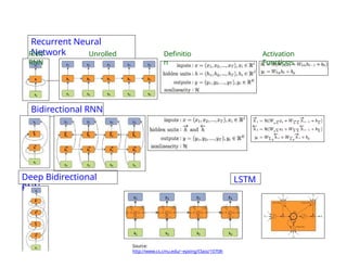
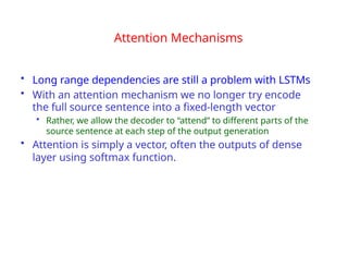
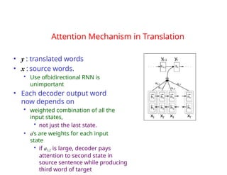
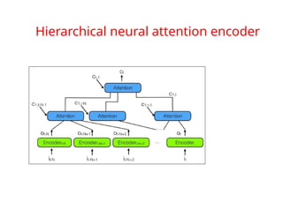
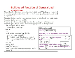
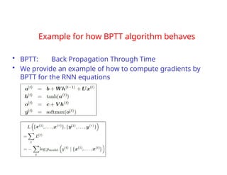
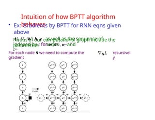
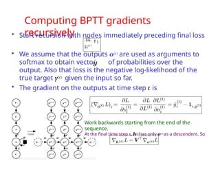
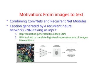
The document provides an extensive overview of sequence modeling with a focus on recurrent neural networks (RNNs) and their various architectures, including bidirectional RNNs and encoder-decoder models. It discusses challenges such as long-term dependencies, optimization techniques like LSTM and attention mechanisms, and applications in natural language processing and machine translation. Additionally, it explores the process of unfolding computational graphs to effectively model recurrent relationships in sequential data.
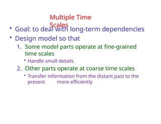
![Two common tasks with sequential
data
1. NLP: Named Entity Recognition
• Input: Jim bought 300 shares of Acme Corp. in 2006
• NER: [Jim]Person bought 300 shares of [Acme Corp.]Organization in [2006]Time
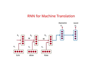
2. Machine Translation: Echte dicke kiste Awesome sauce
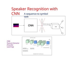
3. Sequence-to-symbol
1. Sentiment:
• Best movie ever Positive
2. Speaker recognition
• Sound spectrogram Harry
1. Sequence-to-sequence
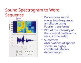
1. Speech recognition using a sound spectrogram
• decompose sound waves into frequency, amplitude using Fourier
transforms
“Nineteenth Century”
Frequencies increase up the vertical axis, and time on the horizontal
axis. The lower frequencies are more dense because it is a male
voice.
Legend on right shows that the color intensity increases with density](https://image.slidesharecdn.com/10-240906023522-5c67a0d9/85/10-0-SequenceModeling-merged-compressed_edited-pptx-5-320.jpg)
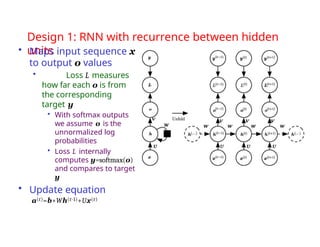
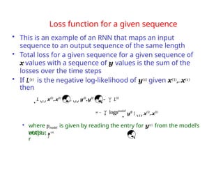
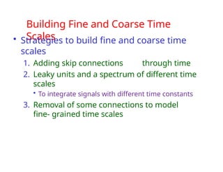
![Loss function for
RNNs
• In feed-forward networks our goal is to
minimize
• Which is the cross-entropy between distribution
of training set (data) and probability distribution
defined by model
• Definition of cross entropy between distributions p and q is
H(p,q)=Ep[-log q]=H(p)+DKL(p||q)
• For discrete distributions H(p,q)=-Σxp(x)log q(x)
• As with a feedforward network, we wish to
interpret the output of the RNN as a probability
distribution
• With RNNs the losses L(t) are cross entropies
between training targets y(t) and outputs o(t)
• Mean squared error is the cross-entropy loss associated
Ex~pˆ data
log
pmodel
(x)](https://image.slidesharecdn.com/10-240906023522-5c67a0d9/85/10-0-SequenceModeling-merged-compressed_edited-pptx-83-320.jpg)


![5G Explained! A High Level Overview [Introduction]](https://cdn.slidesharecdn.com/ss_thumbnails/5gexplainedahighleveloverview-260119165306-cc137a3e-thumbnail.jpg?width=640&height=640&fit=bounds)


