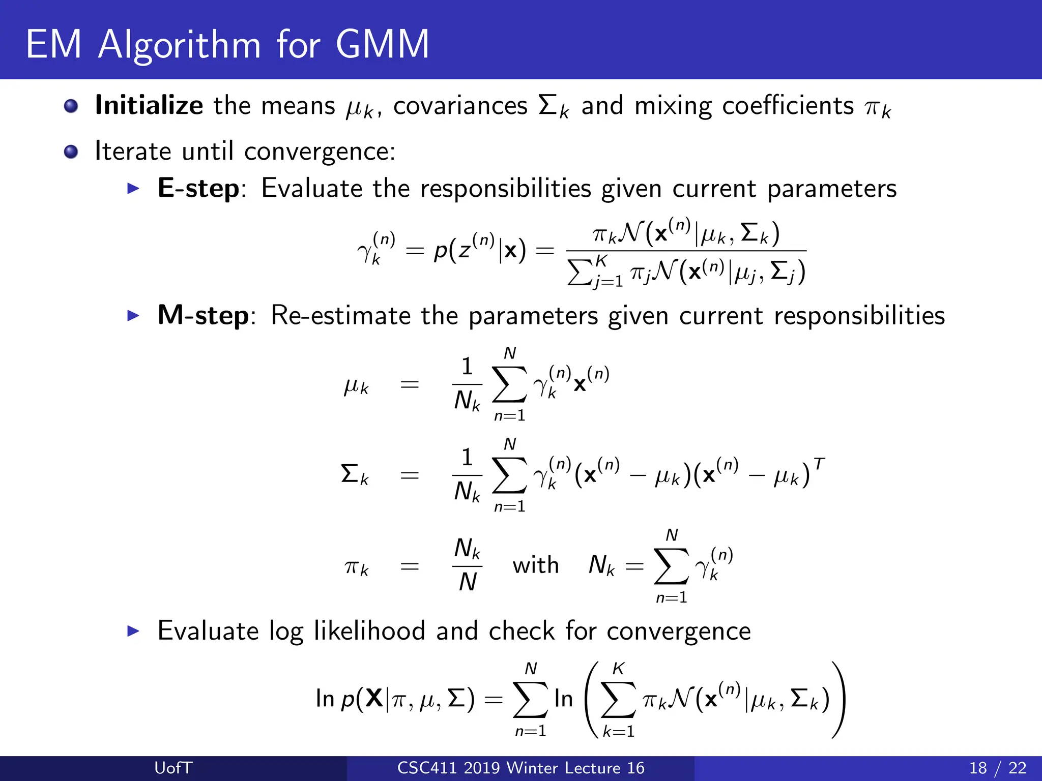
The lecture discusses Gaussian Mixture Models (GMMs) as a statistical method for unsupervised clustering, emphasizing the importance of modeling joint distributions without class labels. It outlines the Expectation-Maximization (EM) algorithm for optimizing GMMs, enabling the handling of latent variables during the clustering of data. GMMs offer a flexible and powerful approach to density estimation, distinguishing it from traditional methods like k-means by using soft assignments instead of hard class assignments.

1. CSC 411: Introduction to Machine Learning
Lecture 16: GMM
Mengye Ren and Matthew MacKay
University of Toronto
UofT CSC411 2019 Winter Lecture 16 1 / 22

2. A Generative View of Clustering
Last time: hard and soft k-means algorithm
This lecture: statistical formulation of clustering → principled, justification
for updates
We need a sensible measure of what it means to cluster the data well
I This makes it possible to judge different methods
I It may help us decide on the number of clusters
An obvious approach is to imagine that the data was produced by a
generative model
I Then we adjust the model parameters to maximize the probability that
it would produce exactly the data we observed
UofT CSC411 2019 Winter Lecture 16 2 / 22

3. Generative Models Recap
We model the joint distribution as,
p(x, z) = p(x|z)p(z)
But in unsupervised clustering we do not have the class labels z.
What can we do instead?
p(x) =
X
z
p(x, z) =
X
z
p(x|z)p(z)
This is a mixture model
UofT CSC411 2019 Winter Lecture 16 3 / 22

4. Gaussian Mixture Model (GMM)
Most common mixture model: Gaussian mixture model (GMM)
A GMM represents a distribution as
p(x) =
K
X
k=1
πk N(x|µk , Σk )
with πk the mixing coefficients, where:
K
X
k=1
πk = 1 and πk ≥ 0 ∀k
GMM is a density estimator
GMMs are universal approximators of densities (if you have enough
Gaussians). Even diagonal GMMs are universal approximators.
In general mixture models are very powerful, but harder to optimize
UofT CSC411 2019 Winter Lecture 16 4 / 22

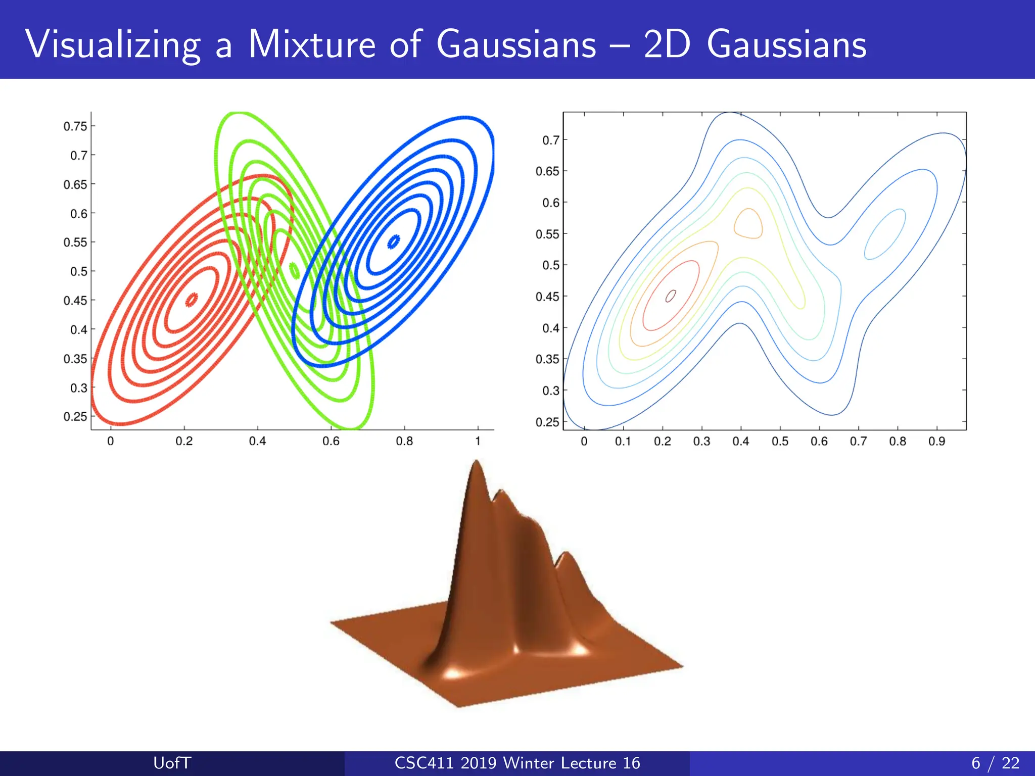
5. Visualizing a Mixture of Gaussians – 1D Gaussians
If you fit a Gaussian to data:
Now, we are trying to fit a GMM (with K = 2 in this example):
[Slide credit: K. Kutulakos]
UofT CSC411 2019 Winter Lecture 16 5 / 22

6. Visualizing a Mixture of Gaussians – 2D Gaussians
UofT CSC411 2019 Winter Lecture 16 6 / 22

7. Fitting GMMs: Maximum Likelihood
Maximum likelihood maximizes
ln p(X|π, µ, Σ) =
N
X
n=1
ln
K
X
k=1
πk N(x(n)
|µk , Σk )
!
w.r.t Θ = {πk , µk , Σk }
Problems:
I Singularities: Arbitrarily large likelihood when a Gaussian explains a
single point
I Identifiability: Solution is invariant to permutations
I Non-convex
How would you optimize this?
Can we have a closed form update?
Don’t forget to satisfy the constraints on πk and Σk
UofT CSC411 2019 Winter Lecture 16 7 / 22

8. Latent Variable
Our original representation had a hidden (latent) variable z which would
represent which Gaussian generated our observation x, with some probability
Let z ∼ Categorical(π) (where πk ≥ 0,
P
k πk = 1)
Then:
p(x) =
K
X
k=1
p(x, z = k) =
K
X
k=1
p(z = k)
| {z }
πk
p(x|z = k)
| {z }
N (x|µk ,Σk )
This breaks a complicated distribution into simple components - the price is
the hidden variable.
UofT CSC411 2019 Winter Lecture 16 8 / 22

9. Latent Variable Models
Some model variables may be unobserved, either at training or at test time,
or both
If occasionally unobserved they are missing, e.g., undefined inputs, missing
class labels, erroneous targets
Variables which are always unobserved are called latent variables, or
sometimes hidden variables
We may want to intentionally introduce latent variables to model complex
dependencies between variables – this can actually simplify the model
Form of divide-and-conquer: use simple parts to build complex models
In a mixture model, the identity of the component that generated a given
datapoint is a latent variable
UofT CSC411 2019 Winter Lecture 16 9 / 22

10. Back to GMM
A Gaussian mixture distribution:
p(x) =
K
X
k=1
πk N(x|µk , Σk )
We had: z ∼ Categorical(π) (where πk ≥ 0,
P
k πk = 1)
Joint distribution: p(x, z) = p(z)p(x|z)
Log-likelihood:
`(π, µ, Σ) = ln p(X|π, µ, Σ) =
N
X
n=1
ln p(x(n)
|π, µ, Σ)
=
N
X
n=1
ln
K
X
z(n)=1
p(x(n)
| z(n)
; µ, Σ)p(z(n)
| π)
Note: We have a hidden variable z(n)
for every observation
General problem: sum inside the log
How can we optimize this?
UofT CSC411 2019 Winter Lecture 16 10 / 22

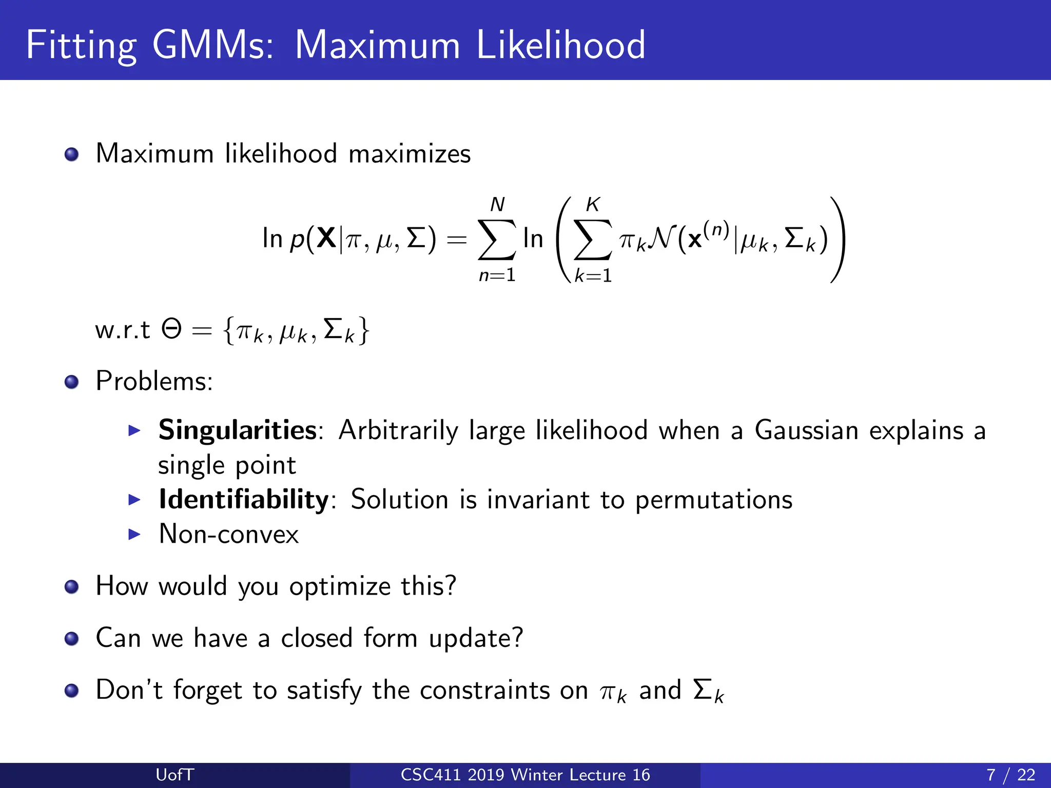
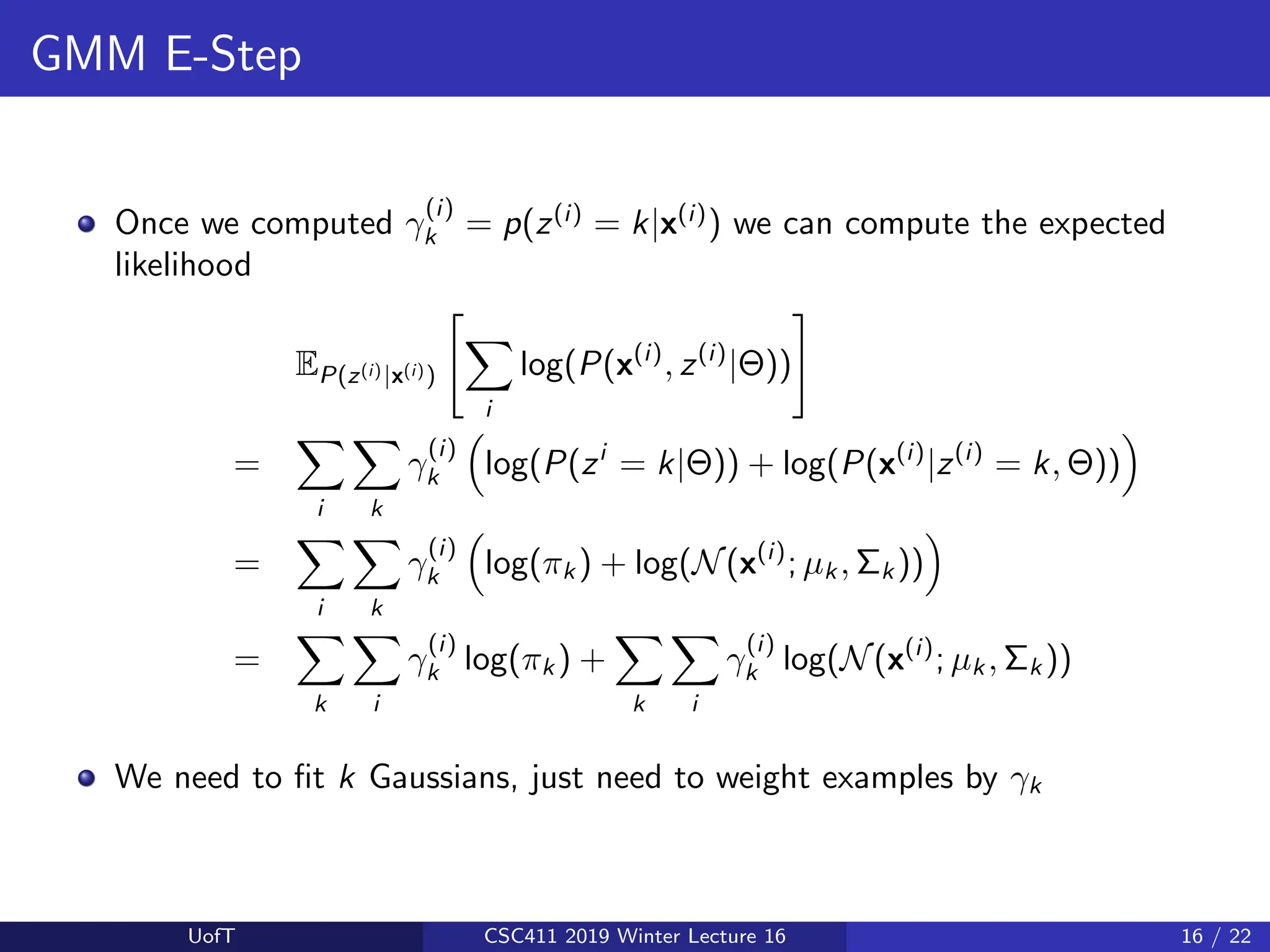
11. Maximum Likelihood
If we knew z(n)
for every x(n)
, the maximum likelihood problem is easy:
`(π, µ, Σ) =
N
X
n=1
ln p(x(n)
, z(n)
|π, µ, Σ) =
N
X
n=1
ln p(x(n)
| z(n)
; µ, Σ)+ln p(z(n)
| π)
We have been optimizing something similar for Gaussian bayes classifiers
We would get this:
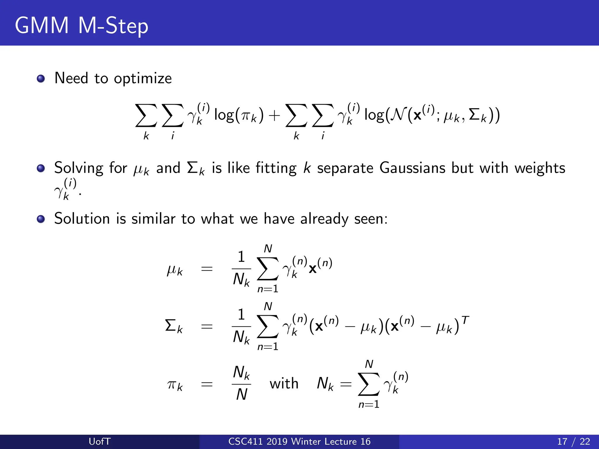
µk =
PN
n=1 1[z(n)=k] x(n)
PN
n=1 1[z(n)=k]
Σk =
PN
n=1 1[z(n)=k] (x(n)
− µk )(x(n)
− µk )T
PN
n=1 1[z(n)=k]
πk =
1
N
N
X
n=1
1[z(n)=k]
UofT CSC411 2019 Winter Lecture 16 11 / 22

12. Intuitively, How Can We Fit a Mixture of Gaussians?
Optimization uses the Expectation Maximization algorithm, which
alternates between two steps:
1. E-step: Compute the posterior probability over z given our current
model - i.e. how much do we think each Gaussian generates each
datapoint.
2. M-step: Assuming that the data really was generated this way, change
the parameters of each Gaussian to maximize the probability that it
would generate the data it is currently responsible for.
.95
.5
.5
.05
.5
.5
.95
.05
UofT CSC411 2019 Winter Lecture 16 12 / 22

13. Relation to k-Means
The K-Means Algorithm:
1. Assignment step: Assign each data point to the closest cluster
2. Refitting step: Move each cluster center to the center of gravity of
the data assigned to it
The EM Algorithm:
1. E-step: Compute the posterior probability over z given our current
model
2. M-step: Maximize the probability that it would generate the data it is
currently responsible for.
UofT CSC411 2019 Winter Lecture 16 13 / 22

14. Expectation Maximization for GMM Overview
Elegant and powerful method for finding maximum likelihood solutions for
models with latent variables
1. E-step:
I In order to adjust the parameters, we must first solve the inference
problem: Which Gaussian generated each datapoint?
I We cannot be sure, so it’s a distribution over all possibilities.
γ
(n)
k = p(z(n)
= k|x(n)
; π, µ, Σ)
2. M-step:
I Each Gaussian gets a certain amount of posterior probability for each
datapoint.
I We fit each Gaussian to the weighted datapoints
I We can derive closed form updates for all parameters
UofT CSC411 2019 Winter Lecture 16 14 / 22

15. GMM E-Step: Responsibilities
Lets see how it works on GMM:
Conditional probability (using Bayes rule) of z given x
γk = p(z = k|x) =
p(z = k)p(x|z = k)
p(x)
=
p(z = k)p(x|z = k)
PK
j=1 p(z = j)p(x|z = j)
=
πk N(x|µk , Σk )
PK
j=1 πj N(x|µj , Σj )
γk can be viewed as the responsibility of cluster k towards x
UofT CSC411 2019 Winter Lecture 16 15 / 22

16. GMM E-Step
Once we computed γ
(i)
k = p(z(i)
= k|x(i)
) we can compute the expected
likelihood
EP(z(i)|x(i))
"
X
i
log(P(x(i)
, z(i)
|Θ))
#
=
X
i
X
k
γ
(i)
k
log(P(zi
= k|Θ)) + log(P(x(i)
|z(i)
= k, Θ))
=
X
i
X
k
γ
(i)
k
log(πk ) + log(N(x(i)
; µk , Σk ))
=
X
k
X
i
γ
(i)
k log(πk ) +
X
k
X
i
γ
(i)
k log(N(x(i)
; µk , Σk ))
We need to fit k Gaussians, just need to weight examples by γk
UofT CSC411 2019 Winter Lecture 16 16 / 22

17. GMM M-Step
Need to optimize
X
k
X
i
γ
(i)
k log(πk ) +
X
k
X
i
γ
(i)
k log(N(x(i)
; µk , Σk ))
Solving for µk and Σk is like fitting k separate Gaussians but with weights
γ
(i)
k .
Solution is similar to what we have already seen:
µk =
1
Nk
N
X
n=1
γ
(n)
k x(n)
Σk =
1
Nk
N
X
n=1
γ
(n)
k (x(n)
− µk )(x(n)
− µk )T
πk =
Nk
N
with Nk =
N
X
n=1
γ
(n)
k
UofT CSC411 2019 Winter Lecture 16 17 / 22

18. EM Algorithm for GMM
Initialize the means µk , covariances Σk and mixing coefficients πk
Iterate until convergence:
I E-step: Evaluate the responsibilities given current parameters
γ
(n)
k = p(z(n)
|x) =
πk N(x(n)
|µk , Σk )
PK
j=1 πj N(x(n)|µj , Σj )
I M-step: Re-estimate the parameters given current responsibilities
µk =
1
Nk
N
X
n=1
γ
(n)
k x(n)
Σk =
1
Nk
N
X
n=1
γ
(n)
k (x(n)
− µk )(x(n)
− µk )T
πk =
Nk
N
with Nk =
N
X
n=1
γ
(n)
k
I Evaluate log likelihood and check for convergence
ln p(X|π, µ, Σ) =
N
X
n=1
ln
K
X
k=1
πk N(x(n)
|µk , Σk )
!
UofT CSC411 2019 Winter Lecture 16 18 / 22

19. UofT CSC411 2019 Winter Lecture 16 19 / 22

20. Mixture of Gaussians vs. K-means
EM for mixtures of Gaussians is just like a soft version of K-means, with
fixed priors and covariance
Instead of hard assignments in the E-step, we do soft assignments based
on the softmax of the squared Mahalanobis distance from each point to
each cluster.
Each center moved by weighted means of the data, with weights given by
soft assignments
In K-means, weights are 0 or 1
UofT CSC411 2019 Winter Lecture 16 20 / 22

21. GMM Recap
A probabilistic view of clustering - Each cluster corresponds to a
different Gaussian.
Model using latent variables.
General approach, can replace Gaussian with other distributions
(continuous or discrete)
More generally, mixture model are very powerful models, universal
approximator
Optimization is done using the EM algorithm.
UofT CSC411 2019 Winter Lecture 16 21 / 22

22. Where does EM come from?
In the next lecture, we’ll see a principled justification of the EM
algorithm and describe how it can be applied to general latent
variable models
UofT CSC411 2019 Winter Lecture 16 22 / 22